TransFusion

Code

Introduction §

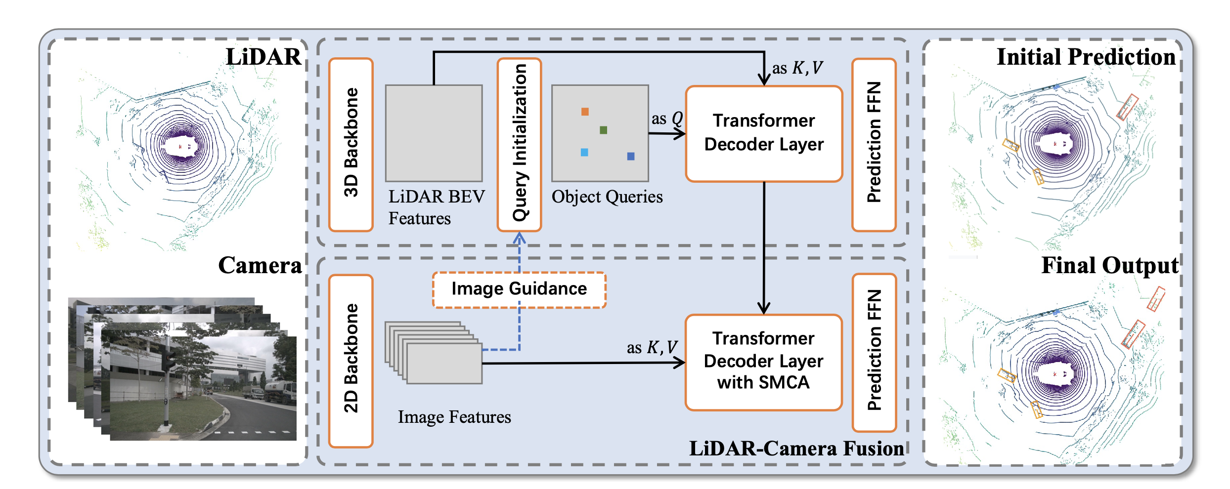
• TransFusion is a lidar-camera fusion with a soft-association mechanism to handle inferior image conditions.
• Introduce adjustments for object queries to boost the quality of initial bounding box predictions for object fusion. Use an image guided system to help detect objects that are difficult to see in point clouds.
• They won 1st place in the nuScenes tracking category.

Existing 2D Work §

• DETR Uses a CNN backbone to extract image features and a transformer architecture to convert a small set of learned embeddings (called object queries) into a set of predictions.
• Further work add positional information to the object queries.
• The final predictions are relative offsets with respect to the query positions to reduce optimization difficulty (vs. having to predict absolute coordinates directly).

Existing 3D Work §

Point cloud only:

• PointNet and PointPillar got good results with only point clouds as input, but they are surpassed by methods using both lidar and camera data.
• Lidar only approaches suffer due to the sparsity of point clouds. Small or distant objects are difficult to detect since they could only recieve a couple points. Those same objects are often still clearly visible and distinguishable in high-resolution images.

Result-level lidar-camera fusion:

• FPointNet and RoarNet are examples.
• They use off-the-shelf 2D detectors to seed 3D proposals followed by a PointNet for object localization.

Proposal-level lidar-camera fusion:

• MV3D and AVOD are examples.
• They perform fusion at the region proposal level by applying ROI Pooling in each modality for shared proposals. This is because each modality generates a proposal for where it thinks an object is. Then, you need to pass the features from each proposal to a downstream network to merge the two, but you need the feature maps to have the same spatial dimensions. In order to get the feature maps of the possibly different bounding boxes to have the same sizes, you need to use RoI Pooling.
• Proposal-level lidar-camera fusion methods show poor results since rectangular regions of interest (RoI) usually contain lots of background noise.

Point-level lidar-camera fusion:

• Find a hard association between lidar points and image pixels based on calibration matrices and then augment lidar features with segmentation scores or CNN features of the associated pixels through point-wise concatenation.
• Another approach is to project both the point cloud and image features into bird’s eye view (BEV) and then fuse the two.

Cons:

• This approach combines features via element-wise addition or concatenation so the performance gets much worse for low-quality image features (ex. images in bad illumination conditions).
• Finding the hard association between sparse lidar points and dense image pixels wastes many image features with semantic information (ex. you might detect the body of an animal but not if its in the sky or on the ground).
• Relies heavily on high-quality calibration between the two sensors.
• You might miss small/distant features if you have a slight miscalibration.

Architecture §

• Consists of convolutional backbones and a detection head based on a transformer decoder.
• The first layer of the decoder predicts initial bounding boxes from a lidar point cloud using a sparse set of object queries (that are input dependent using information from either the lidar BEV and optionally the image features). It takes the object queries as queries and the lidar BEV as keys and values.
• The second decoder layer fuses the object queries (as queries) with useful image features (keys and values). It uses spatially modulated cross attention (SMCA) in the transformer which spatially weights the cross attention.
• The attention mechanism in the transformer allows the model to determine where and what information should be taken from the image leading to an improved fusion strategy.

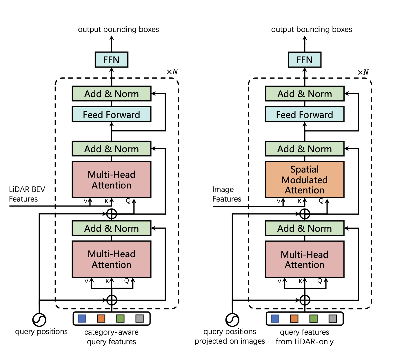
 Left: Architecture of the transformer decoder layer for initial bounding box prediction. Right: Architecture of the transformer decoder layer for image fusion.

First transformer layer §

Inputs:

• Queries: the object queries that are input-dependent and category-aware using features from the lidar BEV and optionally an image BEV. This is different from DETR where the object queries were learned parameters (fixed at inference time).
• Keys/values: the lidar BEV feature map.

Outputs: bounding boxes with initial predictions. Each contains:

• The center offset from the query position, height, length, width, yaw angle, and the velocity.
• It also predicts a per-class probability for $K$ classes.

Design:

• You first compute self-attention between object queries to allow pairwise reasoning of the relationship between different object candidates.
• You compute cross-attention between object queries and the feature maps which aggregates relevant context onto the object candidates.
• The outputs of the multi-head attention ($N$ object queries that are outputted by the last multi-head attention) are passed through an MLP and then eventually through a FFN.

Second transformer layer §

Inputs:

• The initial bounding box predictions from the first transformer layer.
• All image features from the 2D backbone ($F_C\in {\mathbb{R}}^{N_v\times H\times W\times d}$).

Outputs: final bounding box predictions that have been refined from the initial layer and generated using both lidar and image information.

Design:

• Use cross-attention mechanism in the transformer decoder to collect relevant information from the image features onto the initial bounding box predictions.
• Fuses object queries from the first transformer with useful image features (keys, values) associated by spatial and contextual relationships.
• Spatially constrain the cross attention around the initial bounding boxes to help the network better visit the related positions.

Image Feature Fetching:

• Point level fusing approaches (match each lidar point with image data) performs poorly when an object contains only a small number of points so not much image information can be matched to it. To mitigate this issue, TransFusion uses all image features from the CONV backbone $F_C\in {\mathbb{R}}^{N_v\times H\times W\times d}$ and uses this with cross-attention to perform feature fusion.
• Image features are selected by identifying the specific image in which the object queries are located using the previous predictions and calibration matrices. Cross-attention is then performed between the object queries and the corresponding image feature map.

Spatially Modulated Cross Attention (SMCA):

• Lidar and image features are from different domains so the object queries might initially attend to visual regions unrelated to the bounding box. This will result in long training times for the network to accurately identify the proper regions on images.
• TransFusion uses a spatially modulated cross attention which weighs the cross attention by a 2D circular Gaussian mask around the projected 2D center of each query. This is done by element-wise multplying a Gaussian weight mask by the cross-attention map among all the attention heads.
• SMCA results in the network only attending to the related region around the projected 2D box so the network can learn better and faster where to select image features based on the input lidar features.

Query Initialization: §

Unlike input-independent object queries in 2D, they make the object queries input-dependent and category-aware so that the queries are enriched with better position and category information. The queries can either come from the output of the 3D backbone (lidar-only) or a combination of the 2D and 3D backbone output (lidar-camera).

Each object query contains a query position providing the localization of the object and a query feature encoding information such as the box’s size, orientation, etc.

The query initialization was done with either just a heatmap generated from lidar BEV features or using an image-guided approach.

• In earlier works the queries were random or learned as network parameters regardless of the input data. These types of queries require exta layers to move the queries to the real object centers.
• It has been seen in 2D work that a better query initialization strategy could achieve the same performance with a one layer structure as a six layer structure without good initialization.
• TransFusion generates object queries based on a heatmap of object centers. They end up only needing one decoder layer.

Lidar-only query initialization §

Input dependent §

• Takes a $d$ dimensional lidar BEV feature map $F_L\in {\mathbb{R}}^{X\times Y\times d}$ and predicts a class-specific heatmap $\hat{S}\in {\mathbb{R}}^{X\times Y\times K}$ where $X\times Y$ describes the size of the BEV feature map and $K$ is the number of categories.
• This heatmap is used as $X\times Y\times K$ object candidates and the top-N candidates for all categories are selected as the initial object queries.
• To avoid queries that are spatially too close, the local maximum elements (values $\ge$ their 8-connected neighbors) are selected as the final object queries.
• The initial object queries will locate at or close to the potential object centers, eliminating the need of multiple decoder layers to refine the locations.

Category Aware §

• Unlike in 2D detection, objects on the BEV plane are all in absolute scale and have a much smaller variance among objects of the same class.
• The object queries are made category-aware by equipping each query with a category embedding.
• Using the category of each selected candidate (ex. ${\hat{S}}_{ijk}$ belonging to the $k$-th category), they element-wisely sum the query feature with a category embedding produced by linearly projecting the one-hot category vector into a ${\mathbb{R}}^d$ vector. This means they take a one-hot embedding for the category the candidate is predicted to belong to (using the candidate heatmap) and then use a learned network to project that to ${\mathbb{R}}^d$ so it can be combined with the features from the $d$ dimensional lidar BEV feature map.

Benefits:

• Provide useful information when modeling the object-object relations in the self-attention modules and the object-context modules.
• During prediction it can deliver useful prior knowledge of the object and allow the network to focus on intra-category variance.

What's the difference between object-object relations and object-context?

Object-object is when both the keys/values + queries come from the same set of object tokens. Object-context is when one comes from object tokens and one comes from scene tokens.

Image guided query initialization: §

• To leverage the ability of high-resolution images in detecting small objects and make the algorithm more robust against sparse point clouds, they use an image-guided query initialization technique.

Technique:

• Take the image features, $F_C$, that were produced from the 2D backbone ($H\times W\times C$) and collapse the height dimension with a maxpool $(1\times W\times C)$.
• Use the collapsed image features as the keys and values for cross attention with the lidar BEV features $F_L$ that were produced by the 3D backbone as the values.
• The cross attention between the image features and lidar BEV features will produce a lidar-camera BEV feature map $F_{LC}$. Only using cross-attention will save computation cost.
• $F_{LC}$ is then used to predict an object heatmap which is averaged with the lidar-ony heatmap $\hat{S}$ to give the final heatmap ${\hat{S}}_{LC}$.
• Using ${\hat{S}}_{LC}$, the model can detect objects that are difficult to detect with lidar only.

Why collapse the image features from the 2D backbone along the height dimension?

• There is usually at most one object along each image column. Therefore, collapsing along the height axis can significantly reduce the computation without losing critical information.
• Although some fine-grained image features might be lost during this process, it already meets our need as only a hint on potential object positions is required.
• Collapsing the height (instead of the width) was inspired by noticing the relation between BEV locations and image columns can be established easily using camera geometry.
• However, the relation between BEV locations and image rows is more difficult because of occulusion, lack of depth info, unknown ground topology, etc.

Collapsing along height axis §

The dense transformer layer is inspired by the observation that while the network needs a lot of vertical context to map features to the birds-eye-view (due to occlusion, lack of depth information, and the unknown ground topology), in the horizontal direction the relationship between BEV locations and image locations can be established using simple camera geometry. Therefore, in order to retain the maximum amount of spatial information, we collapse the vertical dimension and channel dimensions of the image feature map to a bottleneck of size $B$, but preserve the horizontal dimension $W$. Note: the collapsing is done via a fully-connected network (they don’t just take the max along the columns).

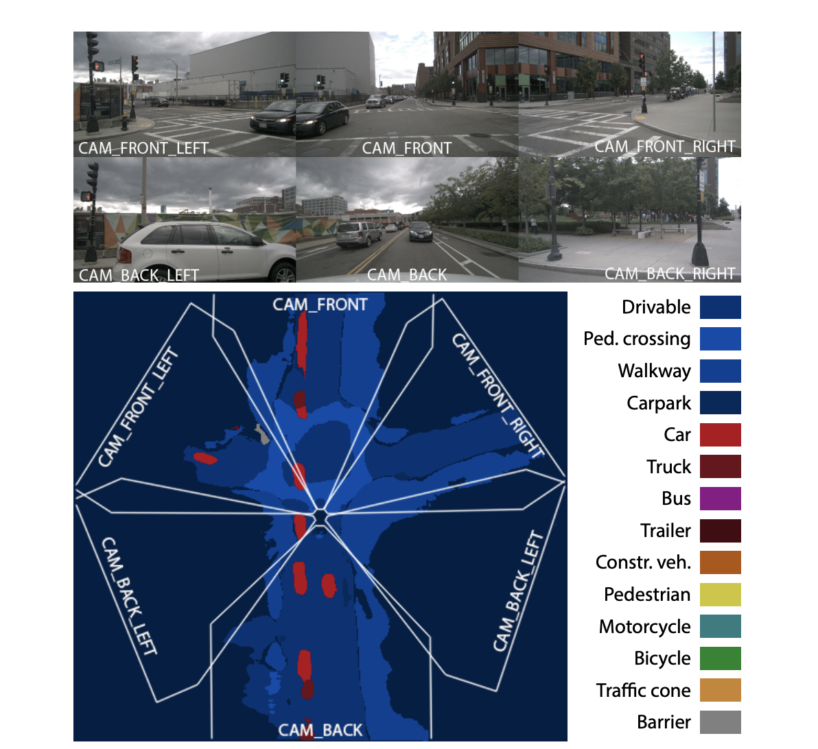
In the image below, you can see it is pretty straight forward to go from the BEV to the front camera column information. However, it is more difficult to decide which row a certain feature should fall into (ex. a car in the distance might be on top of a hill which would place it in a row towards the top of the image).

Figure 3:Our dense transformer layer first condenses the image-based features along the vertical dimension, whilst retaining the horizontal dimension.

Link to original

Label Assignment and Loss §

Matching cost for Hungarian Algorithm §

Like DETR, they use bipartite matching between the predictions and ground truth objects through the Hungarian Algorithm where the matching cost is the weighted sum of classification, regression, and IoU cost: $C_{\text{match }}={\lambda }_1{L}_{cls}(p,\hat{p})+{\lambda }_2{L}_{reg}(b,\hat{b})+{\lambda }_3{L}_{iou}(b,\hat{b})$

• $L_{cls}$ is binary cross entropy loss (this is different from DETR who doesn’t take the log of the probability in order to make the values more comeasurable with the bounding box loss terms).
• $L_{reg}$ is the L1 loss between the predicted BEV and ground-truth centers (normalized between $[0,1]$).
• $L_{iou}$ is the IoU loss between predicted and boxes and ground truth boxes.

DETR’s matching loss is defined as: ${\mathcal{L}}_{\mathrm{match}}\left(y_i,{\hat{y}}_{\sigma (i)}\right)=-1_{\left\{c_i\ne \varnothing \right\}}{\hat{p}}_{\sigma (i)}\left(c_i\right)+1_{\left\{c_i\ne \varnothing \right\}}{\lambda }_{\text{iou }}{\mathcal{L}}_{\text{iou }}\left(b_i,{\hat{b}}_{\sigma (i)}\right)+{\lambda }_{\mathrm{L}1}{\Vert b_i-{\hat{b}}_{\sigma (i)}\Vert }_1$

Loss for matched pairs §

Once the pairs are matched with the Hungarian Algorithm, a Focal Loss is computed for the classification branch. The bounding box regression is supervised by an L1 Loss for only positive pairs. A penalty reduced focal loss is used for the heatmap prediction (see CenterPoint).

The total loss is the weighted sum of losses for each component.