Swin Transformer

Overview §

The Swin Transformer is a hierarchical transformer whose representation is computed with shifted windows. Shifted windows increase efficiency by limiting self-attention to non-overlapping local windows while also allowing for cross-window connections (by shifting the windows for even and odd layers). The model has linear computational complexity with respect to image size (linear with respect to increases in height or width, but not increases in both at the same time) because the self-attention is only within a window. If you divide the image into a grid of 4x4 patches and then increase the width by $w$ you will have $4\times (4+w)=16+4w$ patches to compute and $O(4w)=O(w)$ which is linear with respect to the width.

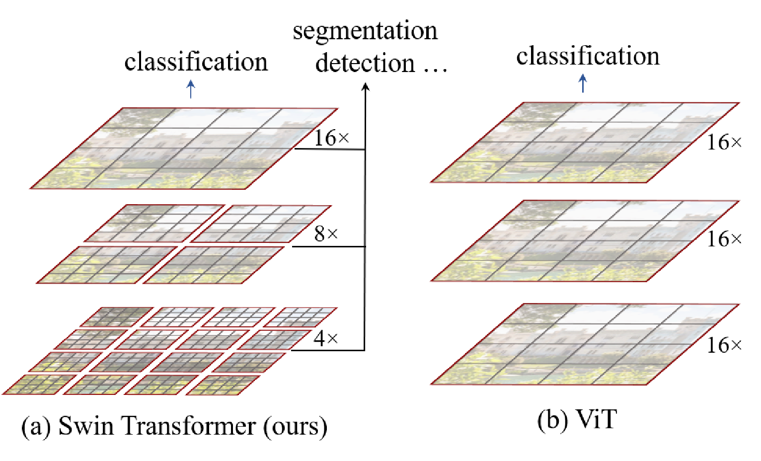
Swin Transformers produce feature maps of varying spatial resolutions, so they can be used as a general-purpose backbone for both image classification and dense recognition tasks by using techniques like feature pyramid networks or U-Net architectures. Swin produces the same resolutions as common CNN architectures (VGG Deeper Networks Regular Design 2014, ResNet) so it can easily replace existing backbones.

Produing a hierarchy of feature maps is done via patch merging layers. Limiting attention to be within a window is seperate and is done to decrease the memory cost of attention. Shifting windows is done to make sure information isn't stuck within a certain area of the grid.

Problems with traditional vision transformers: Traditional vision transformers produce feature maps of a single low resolution and have quadratic computational complexity with respect to the input image size (due to computing self-attention globally).

• Typical transformers are not suitable for things like semantic segmentation because this would require labels on the pixel-level scale which would be quadratic complexity with respect to the image dimensions.
• They also don’t work well for object detection since objects can occur at multiple scales and traditional transformers only produce features at a single scale.

Swin uses a hierarchical architecture unlike traditional ViT

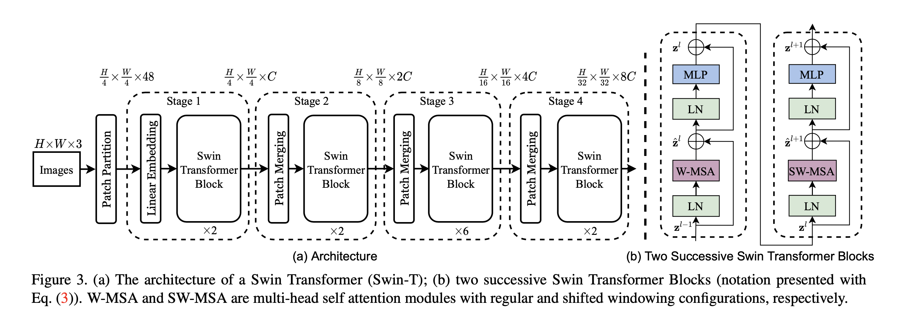
• CNNs process an image in multiple stages. In each stage, the image resolution will be decreased and the number of channels will be increased. This is done with the patch merging layer which groups Cx2x2 patches together, concatenates them to be 4Cx1x1, and then linearly projects them to be 2Cx1x1.
• This is useful since objects in images can occur at various scales. Earlier layers will see higher resolution (and smaller) areas. Later layers will see lower resolution (and larger) areas. This is referred to as multi-scale features.
• In a traditional ViT, all blocks have the same resolution and number of channels (Isotropic Architectures).

Swin Architecture §

First layer of the Swin Transformer §

Like a ViT, the Swin Transformer will start by:

• Take input image of dimension $3\times H\times W$
• Split the image up into patches. However, ViT usually splits the image up into 16x16 pixel regions while a Swin Transformer will split the image up into 4x4 pixel regions. The spatial size of the feature map after the patch embedding will be $3\times \frac{H}{4}\times \frac{W}{4}$ since the image is broken up into 4x4 patches.
• Linearly project each patch to C dimensions using a 1x1 conv (now the feature map is $C\times \frac{H}{4}\times \frac{W}{4}$)
• Have transformer blocks operate on the patches.

Second layer of the Swin Transformer §

The second stage of the Swin Transformer is similar to the first, but introduces a patch merging layer that decreases the spatial resolution by 1/2 in both length and width and double the number of channels.

Patch Merging Layer:

• This will reduce the spatial resolution by merging adjacent patches and increasing the channel dimension.
• You group together a 2x2 section of patches ($C\times 2\times 2$), concatenate the groups to be $4C\times 1\times 1$. The features now have a lower resolution (half the spatial resolution in both height and width), but quadruple the number of channels.
• You then linearly project the $4C$ channels to $2C$ channels with a 1x1 conv.

This layer looks similar to the pooling + projection layers we see at the stage boundaries of ResNet models.

Layers 3,4 §

The third and fourth stage work the same as the second stage. Each stage will reduce the spatial length by 1/2 and increase the number of channels x2. This is now a hierarchial model. After the fourth stage you will have a $8C\times \frac{H}{32}\times \frac{W}{32}$ feature map.

Window Attention §

A typical transformer with a $H\times W$ grid of tokens will have an attention matrix of size $H^2{W}^2$ because you will have an attention score between each pair of entries in the grid of tokens. If you have a 224x224 image with 4x4 pixel patches will result in a spatial grid of size 56x56. The attention matrix will have $56^4=9.8$ million entries.

Problem: computing an attention score between each pair of entries takes up too much memory. Solution: don’t use full attention. Instead, use attention over patches.

Window Attention: Rather than allowing each token to attend to all other tokens, divide the tokens into windows of $M\times M$ tokens (ex. $M=4$ in the video above) and only compute attention within each window.

• The total size of all attention matrices is now $(M^4)(H/M)(W/M)=M^{2}HW$. Note: the $M^4$ comes from each patch of windows being $M\times M$. You then need to flatten these $M\times M$ windows into 1D and this is $M^2$ elements. You then perform a dot-product of these elements by themselves and this is $(M^2{)}^2=M^4$.
• This is linear with respect to image size ($H$ and $W$ for a fixed $M$). This gives a much better scalability for higher resolution images. The Swin Transformer uses $M=7$ throughout the network.

Window Attention Problem: Using window attention, tokens only interact with other tokens within the same window. There is no communcation across windows as you progress through different stages since communication only happens within a window.

Shifted Window Attention §

The solution to the window attention problem is to use shifted window attention. You alternate between normal windows (on even numbered layers) and shifted windows (on odd numbered windows). The shifted windows are shifted over by $\frac{M}{2}$. You will end up with non-square windows at the edges and corners, but you can still implement this efficiently.

Efficient Shifted Window Attention An issue with shifted window partitioning is that it results in more windows and some windows are smaller than $M\times M$. A naive approach to pad the smaller windows to a size of $M\times M$ and mask out the padded values when computing attention results in a considerable increase in computation when the number of windows in regular partitioning is small (as is the case for latter stages in the Swin Transformer since the spatial resolution is reduced).

Swin uses a more efficient batch computation approach by cyclic-shifting toward the top-left as shown below. Here, the shifted windows are re-arranged so that a batched window may be composed of several sub-windows that are not adjacent in the feature map. Masking is used to limit self-attention to within each sub-window.

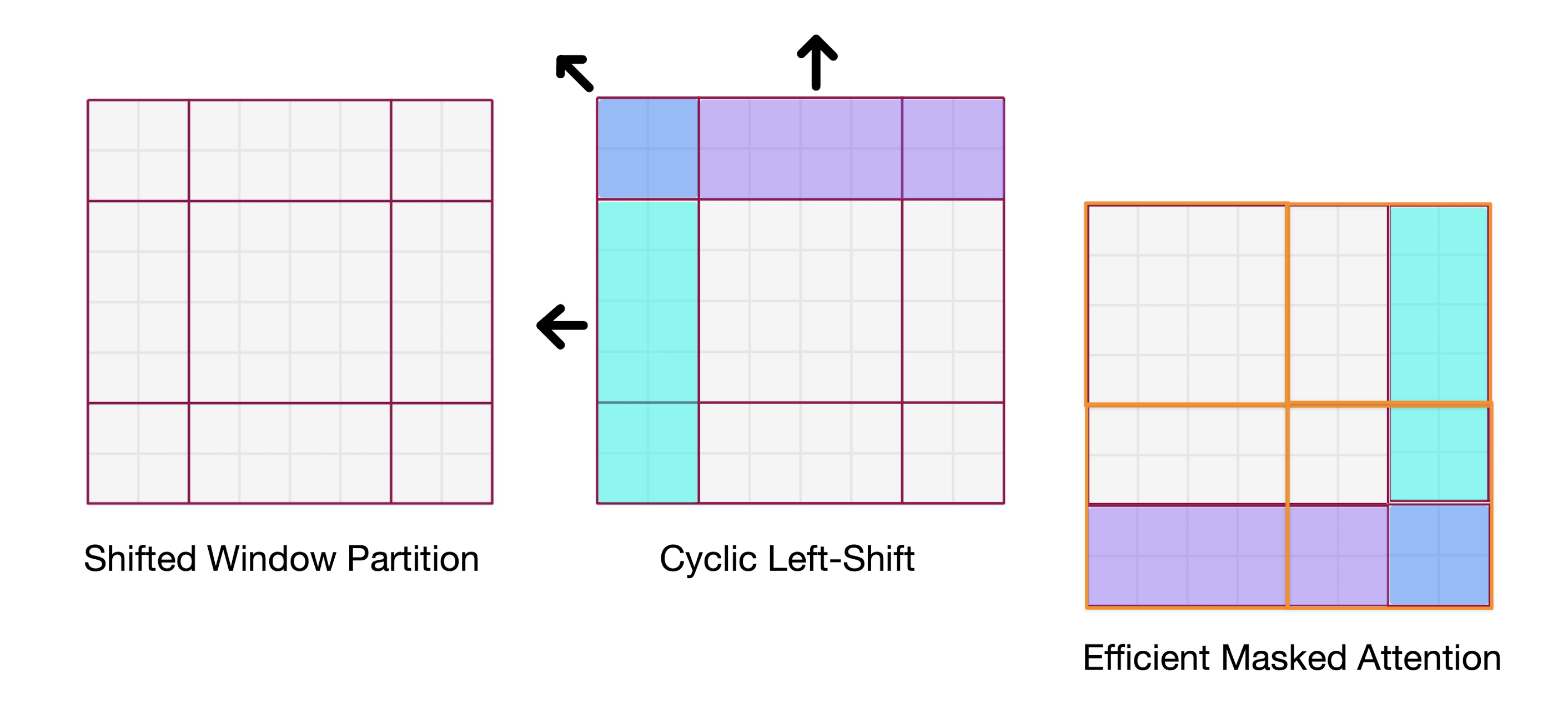
Note that is the windows weren’t cyclic shifted and you just computed masked attention using $M\times M$ windows without shifting you would end up with none of the $M\times M$ windows actually containing an actual window (shown on the left in the diagram below). With the shifted computation, one of the original $M\times M$ windows is preserved and requires no masking.

Relative Positional Bias: §

• ViT models add positional embeddings to the input tokens which encodes the absolute position of each token in the image. This doesn’t work particularly well for the Swin Transformer or vision models since spatial relationships of visual signals are more important vs. absolute position (ex. an animal in the sky vs. ground is important for an image while a noun at the front or end of a sentence tells more about the sentence).
• Swin uses relative positional biases that give the relative position between patches when computing attention.
• ViT/DeiT models abandon translation invariance in image classification even though it has been shown to be crucial for visual modeling. Swin finds that inductive bias encourages certain translation invariance (the model learns to be translationally invariant via the relative positional bias term) is still preferable for general-purpose visual modeling, paticularly for the dense prediction tasks of object detection and semantic segmentation.

Standard Attention: $A=\mathrm{Softmax}\left(\frac{Q{K}^T}{\sqrt{D}}\right)V\text{ where Q,K,V are all M2×D matrices}$

• You take the dot product between the query ($Q$) and key vectors ($K$).
• You then divide by the square root of the dimension ($D$) to compute the scaled dot product attention
• You take the softmax to normalize the un-normalized alignment scores to get the attention weights.
• You multiply the attention weights by the value vector ($V$) to get the output vector.

Attention with relative bias: $A=\mathrm{Softmax}\left(\frac{Q{K}^T}{\sqrt{D}}+B\right)V$ This is the same as above, but you add a learned biases $B$ ($M^2\times M^2$). This is very important for getting good results with the Swin Transformer. Note that you have have a grid of $M\times M$ windows and then you need to flatten this into a sequence of $M^2$ tokens. You then compute self-attention with this sequence which means you have $M^2\times M^2$ positions to account for. The relative position between two patches on each axis lies in the range $[-M+1,M-1]$ (the feature map is split into an $M\times M$ grid of windows so the relative distance between two tokens along an axis can be at most $|M-1|$). Therefore, a ==smaller-sized bias matrix $\hat{B}\in {\mathbb{R}}^{(2M-1)\times (2M-1)}$== is learned and the values for $B\in {\mathbb{R}}^{M^2\times M^2}$ that are used in the attention calculation are taken from $\hat{B}$.

Results §

• Swin Transformer can also be used as a backbone for object detection, instance segmentation, and semantic segmentation. Because they have multiple scales of features, you can use a feature pyramid network to get features at different resolutions. This enables you to do tasks like semantic segmentation (need to detect objects at different scales).
• Swin Transformers don’t need to be trained with distillation unlike other transformers. They can be trained directly on ImageNet.
• Swin Transformers out perform other ViT networks at faster speeds on ImageNet and outperforms even some CNNs.

Related Work §

Other hierarchial vision transformers §

• Swin v2 Fan et al, “Multiscale Vision Transformers”, ICCV 2021
• Multiscale Vision Transformers: Liu et al, “Swin Transformer V2: Scaling up Capacity and Resolution”, CVPR 2022
• Improved MViT: Li et al, “Improved Multiscale Vision Transformers for Classification and Detection”, arXiv 2021

Sliding window approaches to attention for vision: §

• Prajit Ramachandran, Niki Parmar, Ashish Vaswani, Irwan Bello, Anselm Levskaya, and Jon Shlens. Stand-alone self attention in vision models.
• Han Hu, Zheng Zhang, Zhenda Xie, and Stephen Lin. Local relation networks for image recognition.

These approaches used a sliding window approach for attention that suffers from low latency on general hardware due to different key sets for different query pixels. They do this to expedite optimization and achieve slightly better accuracy/FLOPs trade-offs than the counterpart ResNet architecture. However, their costly memory access causes their actual latency to be significantly larger than that of the convolutional networks (need to keep loading different key values). This is in contrast to Swin Transformer where all query patches within a window share the same key set (the windows are shifted between layers vs. doing a sliding window within a layer).

If we take the shifted window example from figure 2 in the paper (below) there are 4 windows. And we just perform self attention locally with the patches within each window.

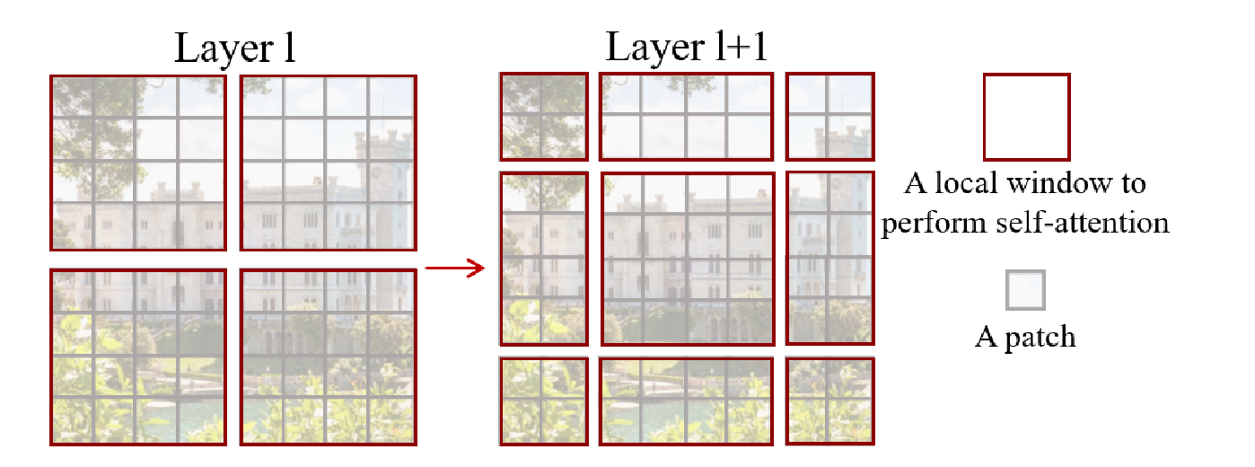
So every patch in one window makes up the queries, keys, and values at the same time. so with 4 windows we do one attention operation in each window. i.e like (softmax(QK))V

In a sliding window approach we might say only one patch at a time is our query (the patch at the center of window at its current position) and the keys are all the patches in the window surrounding the query patch. so naturally the keys would change every time we slide the window to the next query patch which means accessing some new keys every time that window slides and then doing the attention operation at every window position. Source