Normalizing Flows

• Medium Article
• Blog Post
• 1 hour long youtube video
• 15 minute Ari Seff video

What’s the difference between GANs and normalizing flows?

GANs are trained to take a random vector (ex. sampled from Gaussian noise) and produce a data point (ex. an image) via a generator that produces images and a discriminator that judges the quality of these. Normalizing flow models are trained to take a data point (ex. an image) and produce a simple distribution (ex. Gaussian) that minimizes the log-likelihood of the probability of the transformed samples. At inference time for GANs you use the same procedure as for training and sample noise and then pass it to a generator to produce an image. For normalizing flow models, the entire model is invertible so you use a reverse process to what you used during training and sample from noise to produce an image.

Different from autoregressive model and variational autoencoders, deep normalizing flow models require specific architectural structures.

1. The input and output dimensions must be the same.
2. The transformation must be invertible.
3. Computing the determinant of the Jacobian needs to be efficient (and differentiable). This is due to the change of basis formula. See youtube for more details.

Math §

In simple words, normalizing flows is a series of simple functions which are invertible, or the analytical inverse of the function can be calculated.

What is an invertible function

For example, $f(x)=x+2$ is a reversible function because for each input, a unique output exists and vice-versa whereas $f(x)=x^2$ is not a reversible function because both $9$ can correspond to either 3 or -3. The inverse of $f$ exists if and only if $f$ is a Bijective Function (maps each input to exactly one output and vice-versa).

Let $\mathbf{x}$ be a high-dimensional random vector with an unknown true distribution $\mathbf{x}\sim p^{\ast }(\mathbf{x})$. We collect an i.i.d. dataset $\mathcal{D}$, and choose a model $p_{\theta }(x)$ with parameters $\theta$.

In the context of a dataset of images, $\mathbf{x}$ would represent a high-dimensional vector that encodes the pixel values of an image. Each element of the vector corresponds to a pixel in the image, and the dimensionality of the vector is equal to the total number of pixels in the image. The true distribution $p^{\ast }(\mathbf{x})$ would represent the distribution of all possible images that could be generated from the dataset (this is unknown), and the goal of a flow-based generative model would be to learn a model $p_{\theta }(x)$ that can generate new images that are similar to the images in the dataset.

The dataset $D$ being i.i.d. means it is “independent and identically distributed.” In the context of an image dataset, it means that the presence of one image doesn’t affect the probability of the next image and each image has the same likelihood. Stats Stack Exchange Post.

In case of discrete data $\mathbf{x}$, the log-likelihood objective is then equivalent to minimizing:

$\mathcal{L}(\mathcal{D})=\frac{1}{N}{\sum }_{i=1}^N-\log p_{\theta }({\mathbf{x}}^{(i)})$ This is taking the average (summing over all examples and then dividing by the number of examples $N$) of the negative log of the probability that your learned model produces training example ${\mathbf{x}}^{(i)}$.

Optimization is done through stochastic gradient descent using minibatches of data.

In most flow-based generative models the generative process is defined as:

where:

• $\mathbf{z}$ is the latent variable
• $p_{\theta }(\mathbf{z})$ has a simple density (ex. a 0-1 normal distribution).
• ${\mathbf{g}}_{\theta }(\dots )$ is an invertible (aka bijective) function that to produce a latent variable $\mathbf{z}$, you compute $\mathbf{z}={\mathbf{f}}_{\theta }(\mathbf{x})={\mathbf{g}}_{\theta }^{-1}(\mathbf{x})$. This means ${\mathbf{f}}_{\theta }$ is the inverse of ${\mathbf{g}}_{\theta }$.

What is a latent variable?

A latent variable, in the context of statistics and data analysis, is a variable that is not directly observed but is inferred or estimated from other observed variables.

During the training process of the model, you take an image $\mathbf{x}$ and then pass it to the inverse of ${\mathbf{g}}_{\theta }$ which is ${\mathbf{f}}_{\theta }$ (you are learning the model ${\mathbf{f}}_{\theta }$ during training). ${\mathbf{f}}_{\theta }(\mathbf{x})$ then produces $\mathbf{z}$ which is a vector that belongs to the simple density function $p_{\theta }(\mathbf{z})$ you are trying to learn. For instance, if your density function has dimension = 256, then ${\mathbf{f}}_{\theta }$ will produce a vector of dimension = 256 that corresponds to the images representation in the density function space.

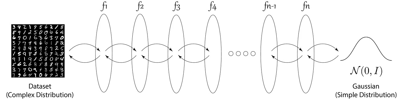
We focus on functions where $\mathbf{f}$ (and, likewise, $\mathbf{g}$) is composed of a sequence of transformations $\mathbf{f}={\mathbf{f}}_1\circ {\mathbf{f}}_2\circ \cdot \cdot \cdot \circ {\mathbf{f}}_K$ such that the relationship between $\mathbf{x}$ and $\mathbf{z}$ can be written as:

$\mathbf{x}\stackrel{{\mathbf{f}}_1}{⟷}{\mathbf{h}}_1\stackrel{{\mathbf{f}}_2}{⟷}{\mathbf{h}}_2\cdots \stackrel{{\mathbf{f}}_K}{⟷}\mathbf{z}$ This just means that you compose a series of invertible functions in a sequence such that you can take $\mathbf{x}$ to $\mathbf{z}$ in a way that you can then perform the inverse computation.

Such a sequence of invertible transformations is also called a (normalizing) flow

Under the change of variables formula, the probability density function (pdf) of the model given a datapoint can be written as:

$\begin{array}{rl}\log p_{\mathbf{\theta }}(\mathbf{x})& =\log p_{\mathbf{\theta }}(\mathbf{z})+\log |\det (d\mathbf{z}/d\mathbf{x})|\\ & =\log p_{\mathbf{\theta }}(\mathbf{z})+\sum _{i=1}^K\log \left|\det \left(d{\mathbf{h}}_i/d{\mathbf{h}}_{i-1}\right)\right|\end{array}$

which means that the log probability of a datapoint $p_{\theta }(x)$ is equivalent to something you can represent in terms of the log probability of the simple distribution of your latent variable $p_{\theta }(\mathbf{z})$.

You can therefore represent the log-likelihood objective you are minimizing as:

$\mathcal{L}(\mathcal{D})=\frac{1}{N}{\sum }_{i=1}^N-\log p_{\theta }({\mathbf{x}}^{(i)})$

which is equivalent to:

$\mathcal{L}(\mathcal{D})=-\frac{1}{N}{\sum }_{i=1}^N(\log p_{\mathbf{\theta }}(\mathbf{z})+{\sum }_{i=1}^K\log \left|\det \left(d{\mathbf{h}}_i/d{\mathbf{h}}_{i-1}\right)\right|)$

which is useful since you can find out the probability of a point from a normal distribution while you couldn’t find out the probability of an image ($p_{\theta }({\mathbf{x}}^{(i)})$) so you can now actually calculate your objective.