DeepLab

Great YouTube Video

DeepLabv1 refers to the original conference paper. DeepLabv2 is the final paper published and includes significant improvements (switched from VGG to ResNet backbone).

Main contributions §

• Highlight atrous convolution (aka dilated convolution) as a useful tool. You can explicitly control the resolution that computation happens within the network because you can change the dilation factor to capture multiple fields of view.
• Propose atrous spatial pyramic pooling (ASPP) to segment objects at multiple scales by probing an incoming feature layer with multiple sampling rates and effective fields of views.
• Improve segmentation accuracy around object borders by combining methods from DCNN (Deep Convolutional Neural Networks) and probabilistic models (a fully connected Conditional Random Field).

Related Work §

Early approaches that use hand-crafted features combined with flat classifiers (Boosting, Random Forests, or SVMs). More modern approaches use CNNs and there are three main groups they fall into.

Use a CNN for image segmentation (predict object region) and then use another CNN for region classification. The object region predictions provide shape information to the secondary network to help the classification process. However, it isn’t possible to recover from incorrect image segmentation regions.

Predict segmentations and CNN features in parallel and then combine results. These works also decouple the segmentation algorithm from the CNN feature extractor results which means you can’t recover from poor CNN features.

Predict per-pixel labels directly. This approach uses a fully convolutional network that directly predicts per-pixel labels. This is the approach that DeepLab uses.

Semantic Segmentation with Traditional CNNs §

Also see Idea 2: Fully Convolutional Networks.

Traditional CNNs have a built-in invariance to local image transformations which allows them to learn abstract data representations. This works well for image classification, but they have some challenges when applied to semantic segmentation since you want sharp borders.

Challenges with using a traditional CNN §

Reduced feature resolution caused by repeated max-pooling and downsampling (with strided convolutions). Traditional CNNs typically are doing image classification. It is okay for them to work at a lower resolution since they just need a global understanding of the image. Additionally, working at a lower resolution is more computationally efficient. However, when you want to do semantic segmentation, you need to work at a higher resolution.

DeepLab addresses this by using Dilated Convolution to keep the spatial resolution large while still increasing the effective field of view and maintaining the same number of parameters and computation. They also use bilinear interpolation later in the network to go up from a downscaled version of the image back to the original resolution.

Existence of objects at multiple scales. Objects can appear at multiple scales within an image. The standard way to deal with this is to provide the same image at different scales to the network and then aggregate the resulting features. This improves performance, but it comes at the cost of computing feature responses at all network layers for multiple scaled versions of the input image.

Instead of passing multiple scales of the input image, DeepLab resamples a given feature layer at multiple rates prior to convolution. This is similar to applying multiple filters to the original image that have complementary effective fields of view, thus capturing objects as well as useful image context at different scales.

Instead of resampling the features directly, this is implemented by using parallel dilated convolution layers with different dilation rates. This is called atrous spatial pyramid pooling (ASPP).

Reduced localization accuracy due to invariance 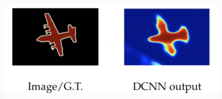The above shows that the borders are very blurred. Small differences in the input image don’t have a big effect on the output due to downsampling and maxpooling present in most CNN networks.

A classifier made for object classification requires invariance to spatial transformations (a picture of a cat is still a picture of a cat even if the cat is in a different location). This is achieved by downsampling and maxpooling. The standard approach to handle this is to use skip-connections to make use of information from multiple network layers.

DeepLap instead boost’s the model’s ability to capture fine details by using a fully-connected Conditional Random Field. CRFs have been used in semantic segmentation to combine class scores computed by multi-way classifiers (predict over a set of labels where the confidence sums to 1) with the lowlevel information captured by the local interactions of pixels and edges.

DeepLab couples a deep convolutional neural network that provides pixel-level classification with the CRF. Note that the CRF runs on CPU.

Architecture §

A deep convolutional neural network (VGG-16 or ResNet-101 in this work) trained in the task of image classification is re-purposed to the task of semantic segmentation by:

1. transforming all the fully connected layers to convolutional layers (i.e., fully convolutional network) and
2. increasing feature resolution through dilated convolutional layers, allowing us to compute feature responses every 8 pixels instead of every 32 pixels in the original network. Bilinear interpolation is then used to upsample by a factor of 8 the score map to reach the original image resolution, yielding the input to a fully connected CRF that refines the segmentation results.

Dilated Convolution §

Note

Dilated convolutions allow you to control the field-of-view and finds the best trade-off between accurate localization (small field-of-view) and context assimilation (large field-of-view).

Fully Convolutional Networks for Semantic Segmentation uses deconvolution layers (upsample with learned parameters), but this requires additional memory and time (additional layers to backprop through).

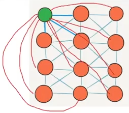
DeepLab uses Dilated Convolutions (shown above where the 3x3 filter is applied to the blue input with gaps inserted between the elements it is applied to). You can use dilated convolutions in a chain of layers which allows you to compute the final network responses at any resolution (up to the original image resolution).

DeepLab replaces the traditional Conv layers in ResNet and VGG with dilated convolutions to increase the spatial resolution by a factor of 4 and then uses bilinear interpolation to increase the resolution by a factor of 8 to recover the feature maps at the original image resolution. Unlike the deconvolution approach used by Fully Convolutional Networks for Semantic Segmentation, this approach doesn’t require any additional learnt parameters.

Atrous Spatial Pyramid Pooling (ASPP) §

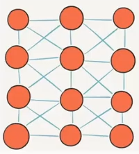
It’s a common theme in CNN’s to have a block that concatenates the features from multiple parallel convolution pathways with different field of views (example below is from Inception Networks) 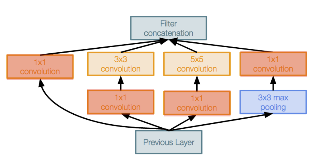Instead of using multiple convolutional layers, DeepLap just uses one convolutional kernel with different distillation rates to capture multiple FOVs.

The paper experimented with different FOVs in the ASPP module and the larger the FOVs, the better the results.

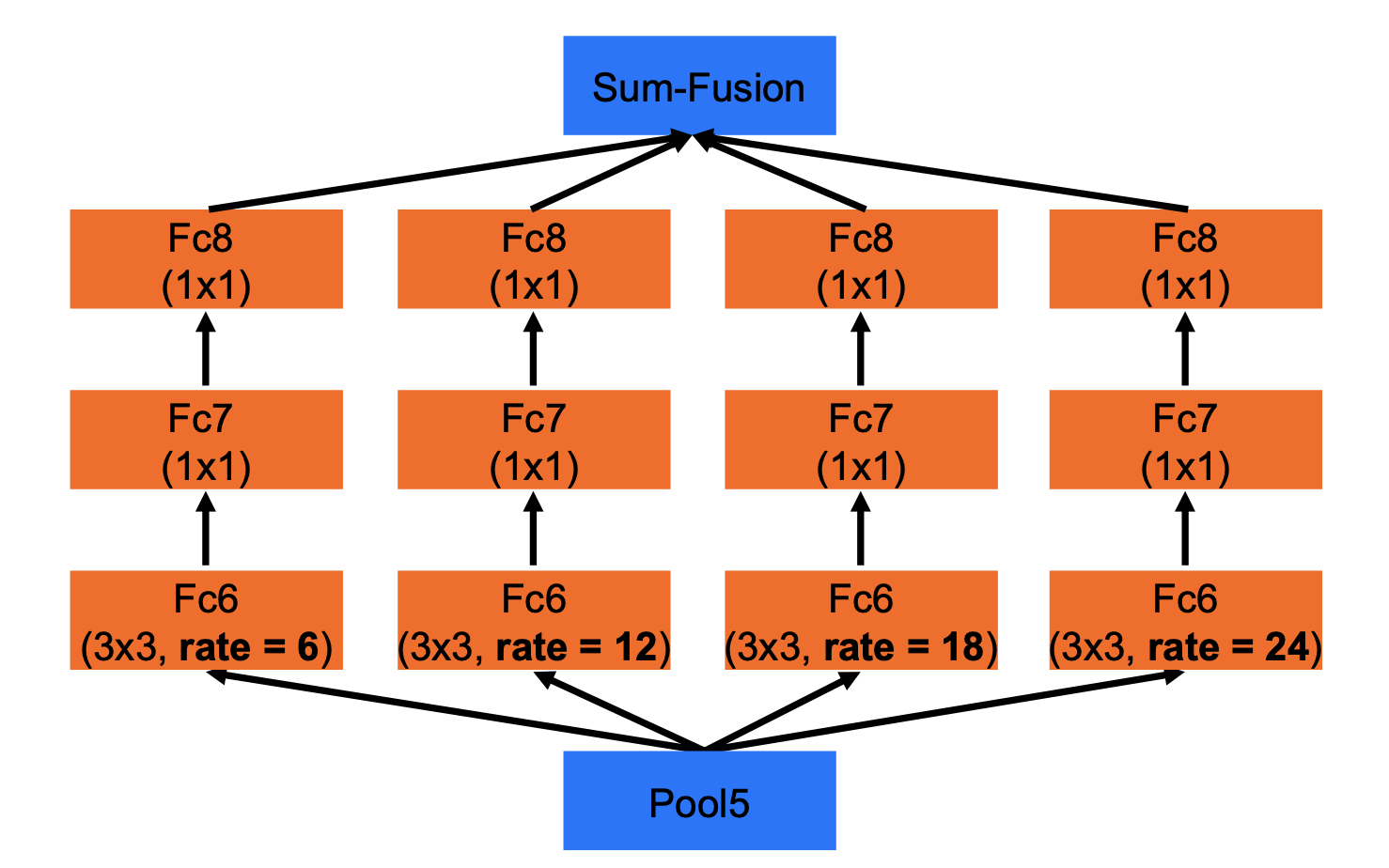
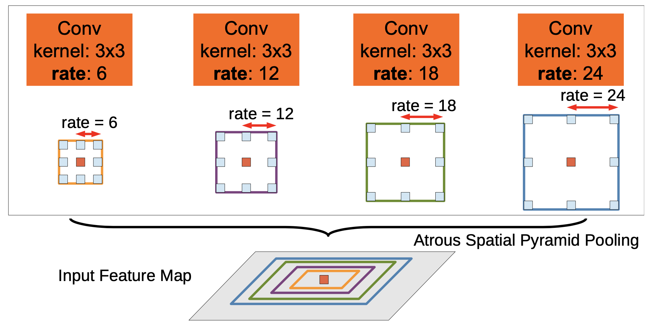In the example above, to classify the classify the center pixel (orange), ASPP exploits multi-scale features by employing multiple parallel filters with different rates. The effective Field-Of-Views are shown in different colors.

ASPP encodes objects and image context at multiple scales without requiring recomputing feature responses at all CNN layers for multiple scales of input.

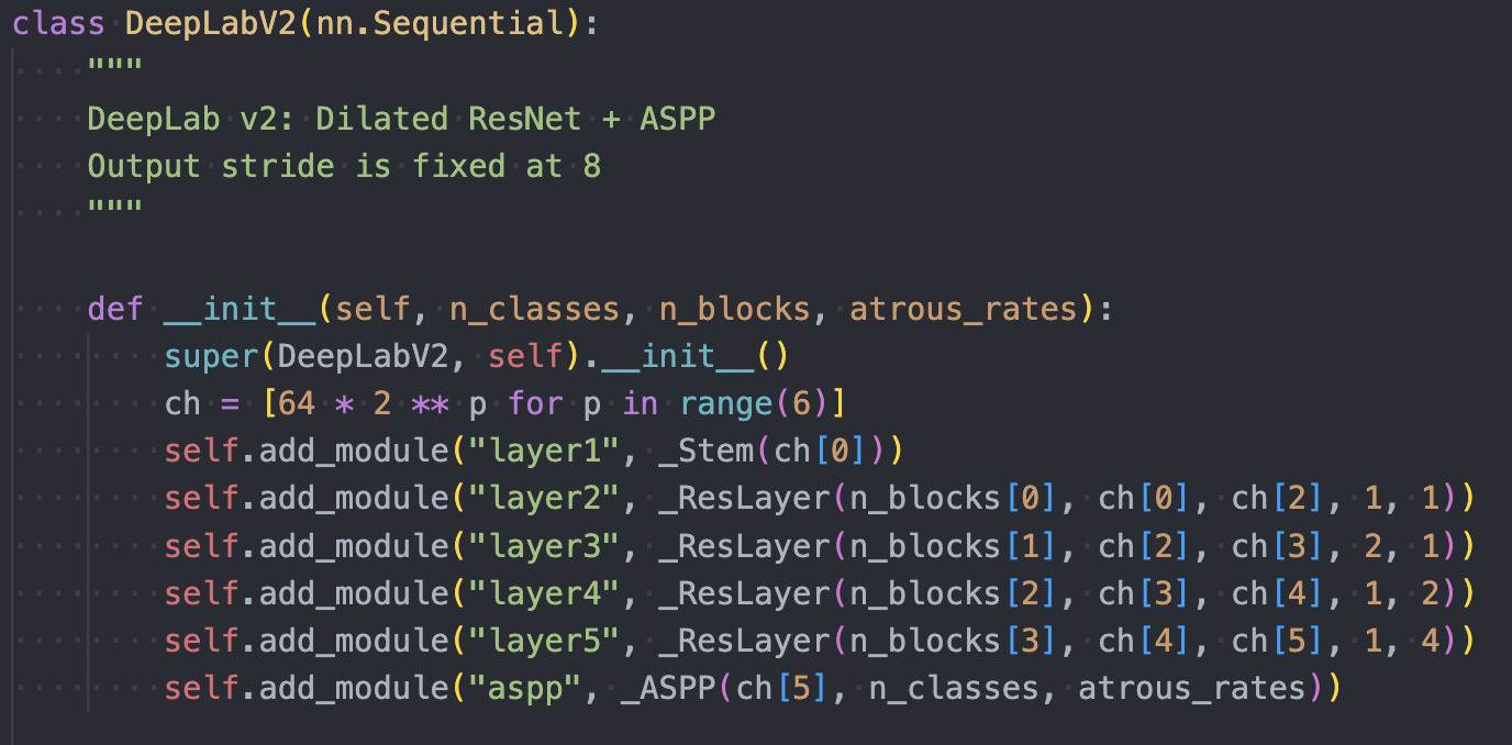
DeepLab adds the ASPP layer as the head of the model: 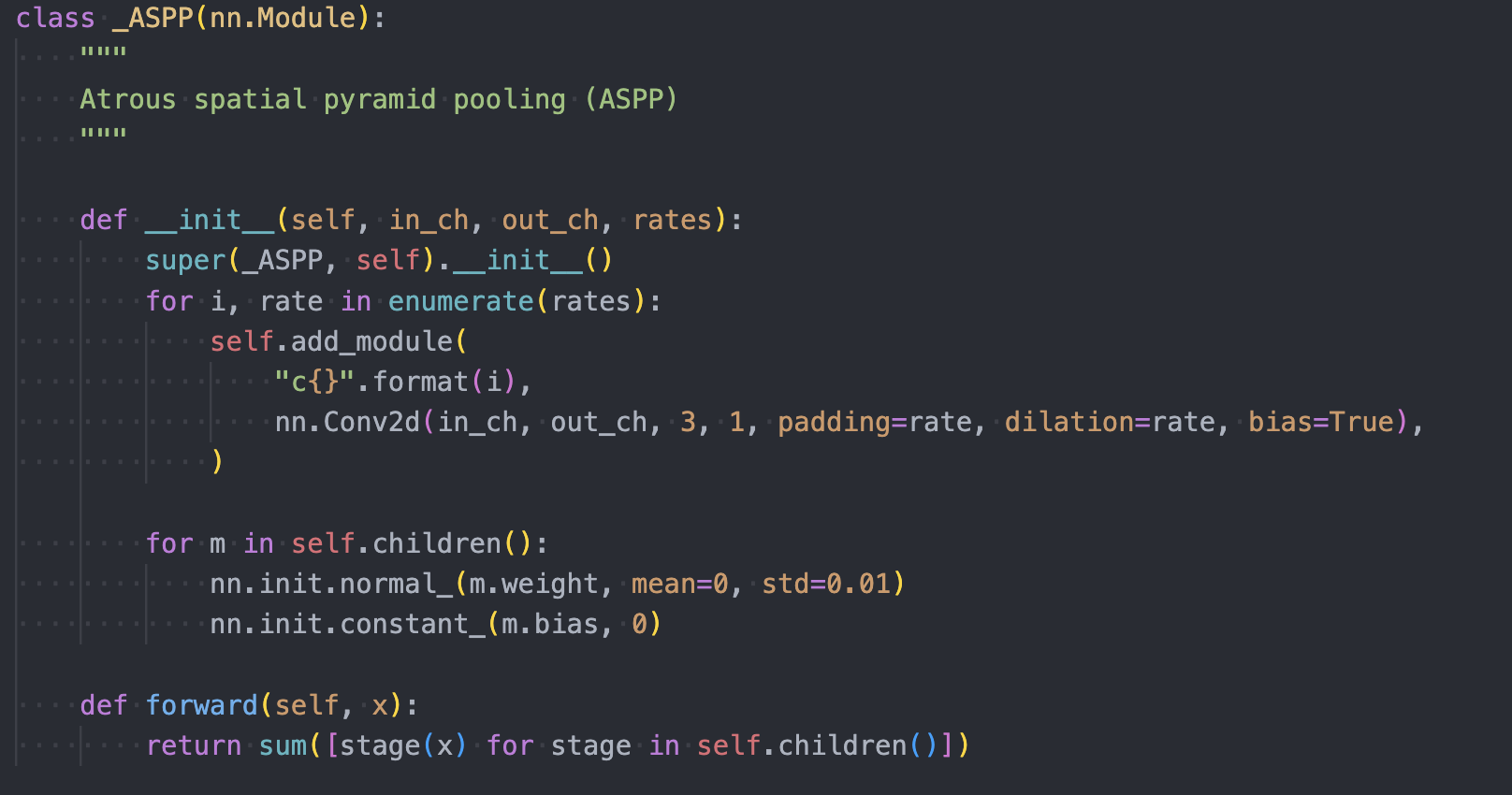which is then used via:

Conditional Random Fields (CRFs) §

Deeper CNNs have more max-pooling layers and downsampling and although they perform better for classification, the increased invariance and the large receptive fields of latter layers can only yield smooth responses (hard to get sharp boundaries). This motivated the paper to try to use CRFs to improve boundary predicition.

These are probabilistic models that treat the pixels in the image as a graph. Using CRFs isn’t a new idea, but previously mostly short-range or locally connected CRFs were used (you connect each pixel to its neighboring pixels). DeepLab instead uses a fully-connected CRF (connect each pixel to all other pixels).

Why were local CRFs previously used?

Traditionally CRFs have been used to smooth noisy segmentation maps that were produced by weak classifiers built on hand-engineered features. These outputs were noisy and the CRFs were used to smooth the noise.

Current CNNs are deeper and the borders are already blurred so using local CRFs would only further blur these boundarires. Therefore, a fully connected CRF is used by DeepLab.

On the left is a local CRF and on the right is a fully-connected CRF.

The CRF optimization function is setup such that:

• There is no penalty is if the pixels have the same label.
• There is a large penalty if the pixels are close together and have similar intensities.
• There is a small penalty if the pixels are far from each other and have different intensities. This is because you want the CRF to focus on improving accuracy around borders where pixels are close together and often have similar intensities.

Updating ResNet to increase spatial resolution §

The paper describes their method to update a single layer as:

In order to double the spatial density of computed feature responses in the VGG-16 or ResNet-101 networks, we find the last pooling or convolutional layer that decreases resolution (pool5 or conv5_1 respectively), set its stride to 1 to avoid signal decimation, and replace all subsequent convolutional layers with atrous convolutional layers having rate r = 2.

This process is then repeated for as many previous layers as needed until the desired output resolution is achieved.

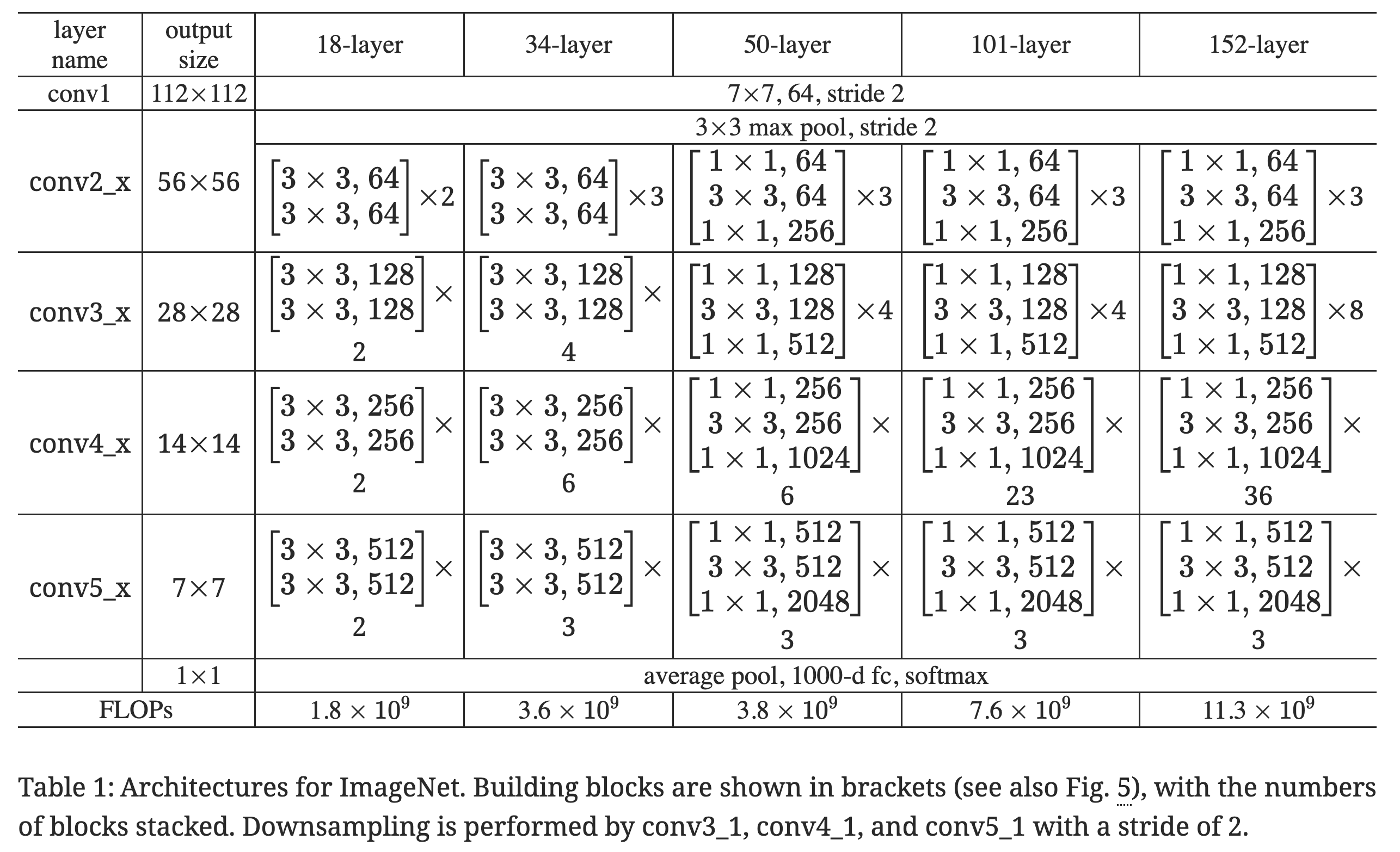DeepLab uses ResNet101 as their backbone. This will downsample via stride=2 in the first 3x3 convolution in the first block in layers conv3, conv4, and conv5. Using stride=2 will decrease the spatial resolution in half (ex. the input to conv5 is $14\times 14$ and the output from conv5_1 is $7\times 7$).

“Set its stride to 1 to avoid signal decimation” just means that they change the stride from 2 to 1 for the last convolution layer that decreases spatial resolution (conv5_1) so the spatial resolution isn’t decreased by this layer (it remains $14\times 14$ after conv5_1).

Since the spatial resolution isn’t reduced by 1/2, you need to set the dilation rate to 2 for all layers after the Conv2D you changed the stride for. This is because all these layers’ kernels have weights that were trained with an input with 1/2 the spatial resolution you are now passing to them. Since you changed stride=2 to stride=1, the inputs to these layers will now have twice the original spatial resolution. In order to handle this, you set the distillation rate = 2 so that the kernels skip pixels in the input and you can use the same kernels while keeping the spatial resolution x2 what it originally was (you will be applying the filter additional times to cover the larger input).

You then need to repeat this process again and update conv4’s stride to 1. This is because you want to the final output to be downsampled 8x from the input image (vs. the original 32x downsampling from ResNet). This requires not downsampling by a factor of 32/8 = 4, so you need to remove stride=2 from two layers.

Note

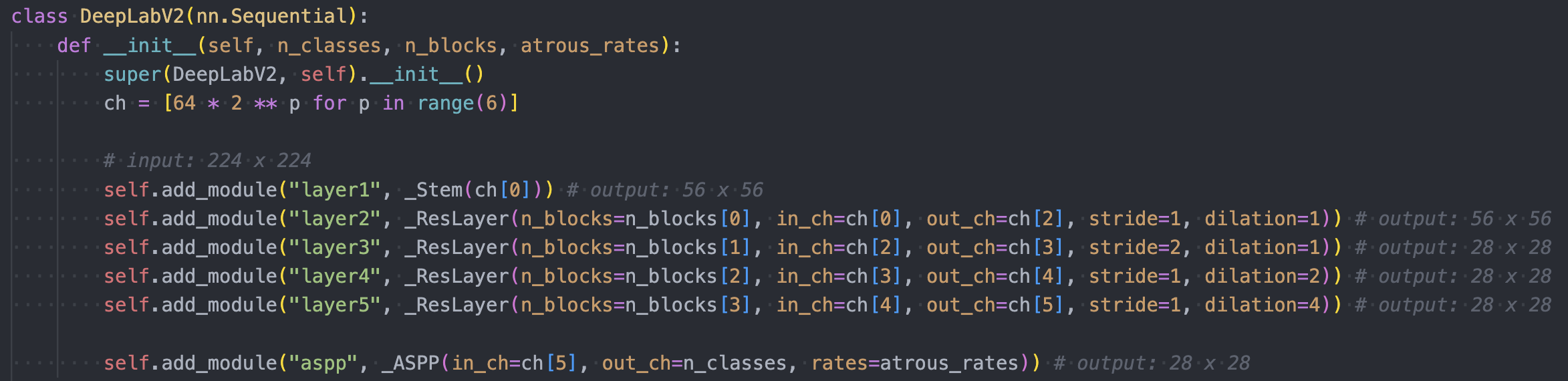
For DeepLab, the last two layers are modified to have stride=1 and dilation=2 for layer4 and dilation=4 for layer5. This results in the output_stride being 32 / (2 * 2) = 8. Therefore, the output resolution is $28\times 28$ instead of $7\times 7$.

The network ends up looking like: where the original ResNet looks like: 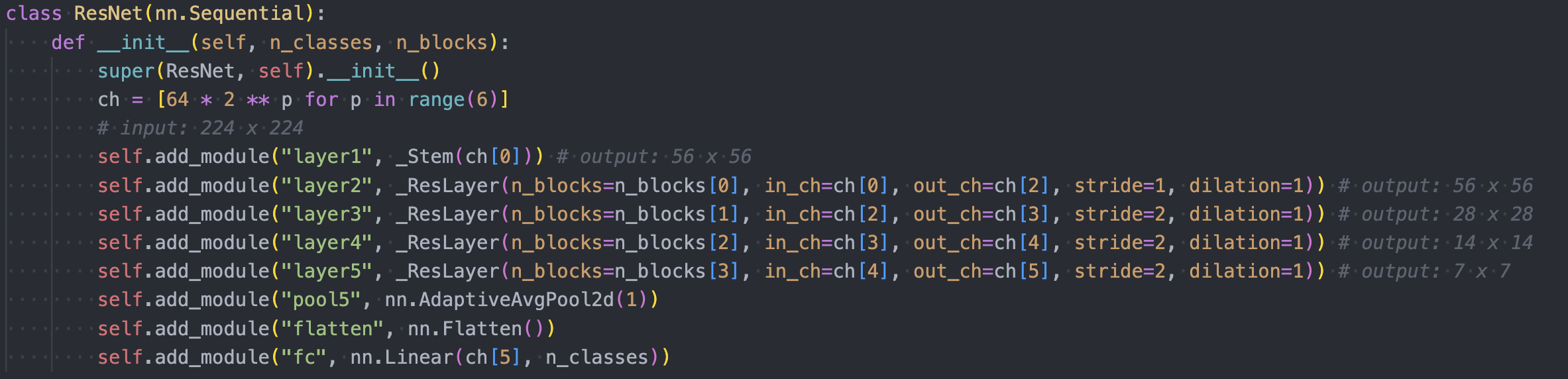DeepLabV2 source and ResNet Source

In order to have outputs downsampled 8x (vs. 32x), you need to change the stride in conv4 and conv5 and set the dilation rates to 2 and 4 respectively.

Ex. for layer4 above you set stride=1 and dilation=2. For the first nn.Conv2D in this layer, you maintain the same FOV as it had with stride=2 by increasing the dilation to 2. For all other nn.Conv2D in this layer, they will have stride 1 (in ResNet only the first nn.Conv2D can have stride > 1). However, they will have dilation=2 since the outputs from the first nn.Conv2D are at a higher spatial resolution.

Summary §

DeepLab Benefits §

1. Algorithm runs fast (or at least it did at time of publishing).
2. Achieved good results on multiple datasets.
3. Simple composition of two well established modules (DCNNs and CRFs).

Results §

• Using ResNet is better than VGG.
• Using CRFs improved performance (note DeepLabv3 doesn’t use CRFs but v1 and v2 do).
• A larger FOV in the ASPP modules improved performance.
• The model couldn’t capture delicate boundaries (ex. bicycles and chairs). The paper hypothesizes using an encoder-decoder structure could be beneficial by making use of the high resolution feature maps passed from the encoder to the decoder.