Implicit Occupancy Flow Fields for Perception and Prediction in Self-Driving

This paper predicts whether a location is occupied and the direction of movement of a location. Previous approaches either detect objects and then predict where the objects are going or predict a dense occupancy and flow grids for the whole scene. This paper instead represents occupancy and flow with a single neural network and can be queried at continuous spatiotemporal locations. Additionally, they avoid the limitations of limited receptive fields from convolutions by using Attention (specifically deformable convolutions and cross attention).

The paper was inspired by implicit geometric reconstruction models which train a neural network to predict a continuous field that assigns a value to each point in a 3D space so that a shape can be extracted as an Iso-surface.

The paper trains an implicit neural network that can be queried for both scene occupancy and motion at any 3-dimensional continuous point $(x,y,t)$ where $x,y$ are spatial coordinates in BEV and $t=\bar{t}+\Delta t$ is the time into the future and $\bar{t}$ is the current time step. $\Delta t\ge 0$ is an offset from the current timestep into the future.

Existing Approaches §

Both of the following approaches have the downside that you need to perform predictions in regions that might be irrelevant for hero.

Object detection + trajectory prediction §

This approach first detects objects in the scene and then predicts trajectories for each object. Since there are multiple possible future trajectories, you need to either generate a fixed number of modes with probabilities or draw samples from the possible trajectory distributions.

Downsides: Uncertainty is not propagated from perception to downstream prediction if you sample discrete samples from the trajectory distributions.

The number of predicted trajectories for each object needs to be limited since it will grow linearly with the number of detected objects in a scene.

For efficiency reasons, only a certain number of objects/objects with a certain confidence are kept. This poses safety concerns as planner is blind to objects below the confidence threshold.

Dense occupancy and flow grids §

This is like what SafetyNet does where you predict a dense grid of occupancy and flow (velocity) at discrete time steps based on sensor data. This is also similar to what FIERY does with the addition of instance tracking. Occupancy Flow Fields adds in backwards flow as a representation that can capture multi-modal forward motions with just one flow vector prediction per grid cell.

This has a benefit over object detection + tracking that you don’t need to threshold objects and the computation doesn’t scale with the number of agents in a scene.

Downsides

• This has the downside that you end up wasting a lot of resources predicting a dense grid since the grid must be very fine to mitigate quantization errors.
• This also suffers from the limited receptive field of CNNs and dividing both the spatial and temporal dimensions into discrete values could result in quantization errors.

Benefits of a query-based approach §

• The model is agnostic to the number of objects in the scene since it predicts the occupancy probability and flow vectors at desired spatio-temporal points instead of per-object (i.e., no issues with too many pedestrians in a scene).
• Using global attention and query points avoids issues with the limited receptive fields of fully convolutional networks. This reduces computation to only that which matters to downstream tasks.
• You can evaluate a large collection of spatio-temporal query points in parallel.

Model §

The model can be represented by $\hat{\mathcal{O}},\hat{\mathcal{F}}=\psi (L,M,\mathcal{Q})$.

Model Inputs §

• The model takes a voxelized lidar representation $L$, a rendered HD map $M$, and a mini-batch $\mathcal{Q}$ containing spatio-temporal query points $\mathbf{q}$.
• The lidar data contains the height for each pixel for the last 5 most recent sweeps.

Model outputs §

For each temporal point, the model will predict the occupancy and flow.

• Let $q=(x,y,t)\in {\mathbb{R}}^3$ be a spatio-temporal point in BEV at future time $t$. The task is to predict the probability of occupancy $o\in [0,1]$ and flow vector ${\mathbb{R}}^2$ specifying the BEV motion of any agent that occupies that location.
• The paper uses Backwards Flow as it can capture multi-modal forward motions with a single reverse flow vector per grid cell.

Model Architecture Overview §

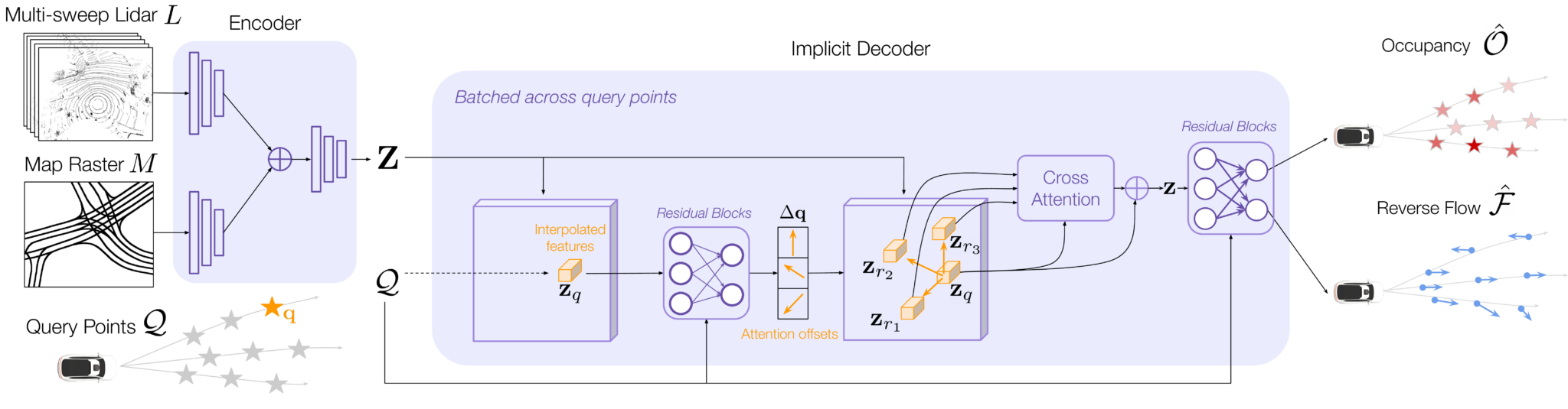The network is divided into a convolutional encoder that computes scene features and an implicit decoder that outputs the occupancy-flow predictions.

Encoder §

• Two convolutional stems process the BEV lidar sweeps and the HD map independently.
• A ResNet then takes the concatenated features and outputs multi-resolution feature maps.
• A lightweight FPN then processes the feature maps and gives a BEV feature map at half the resolution of the inputs $\mathbf{Z}\in {\mathbb{R}}^{C\times \frac{H}{2}\times \frac{W}{2}}$ that contains features capturing the geometry, semantics, and motion of the scene.
• Every feature location contains spatial information about its neighborhood (depending on the size of the receptive field of the encoder) as well as temporal information over the past $T_{\text{history}}$ seconds.

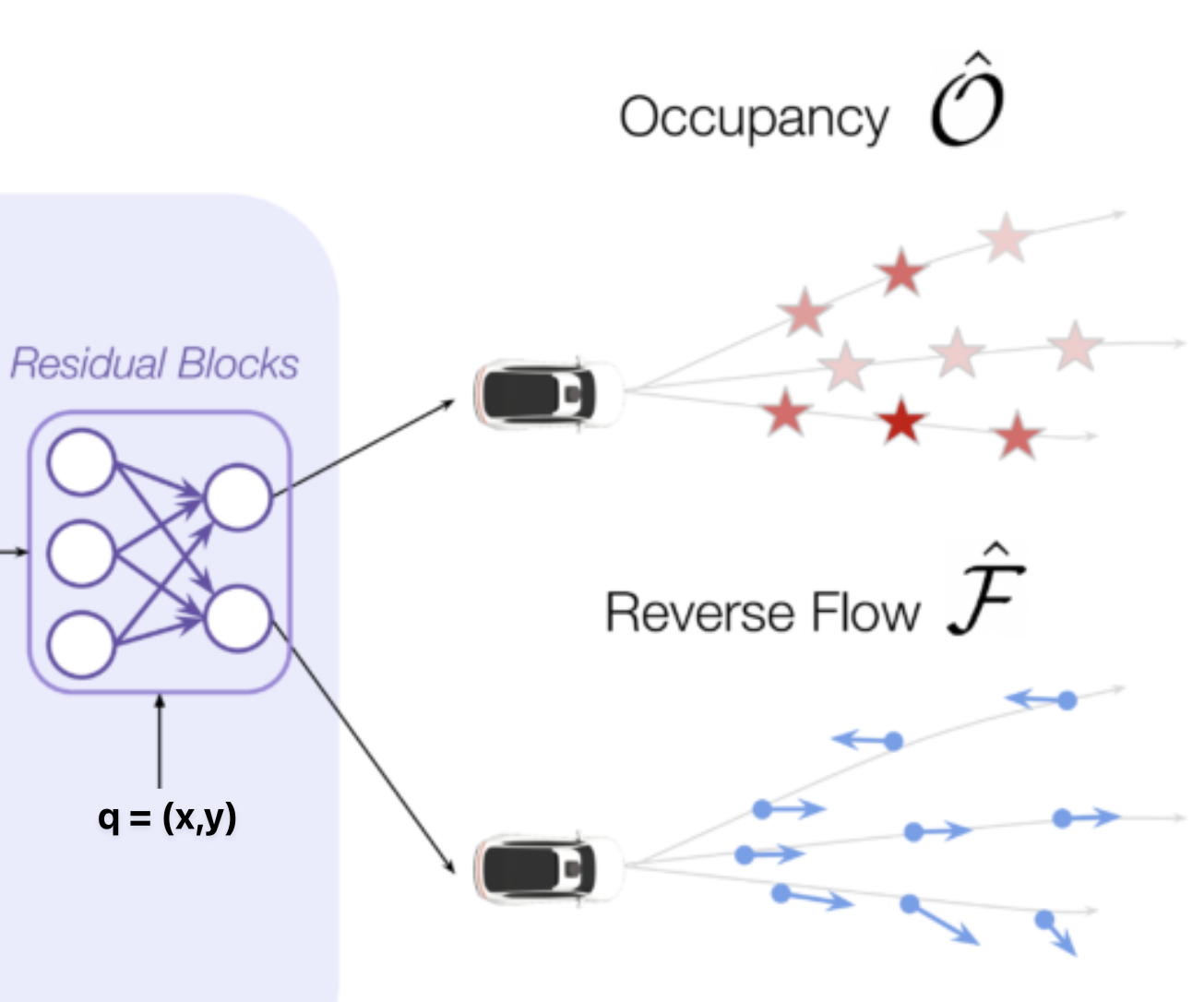
Decoder §

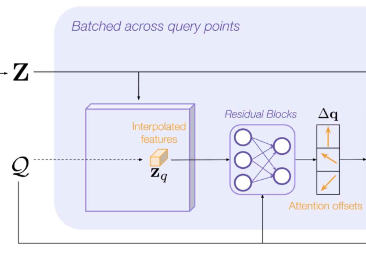
The decoder runs in parallel across queries. For each query, the decoder:

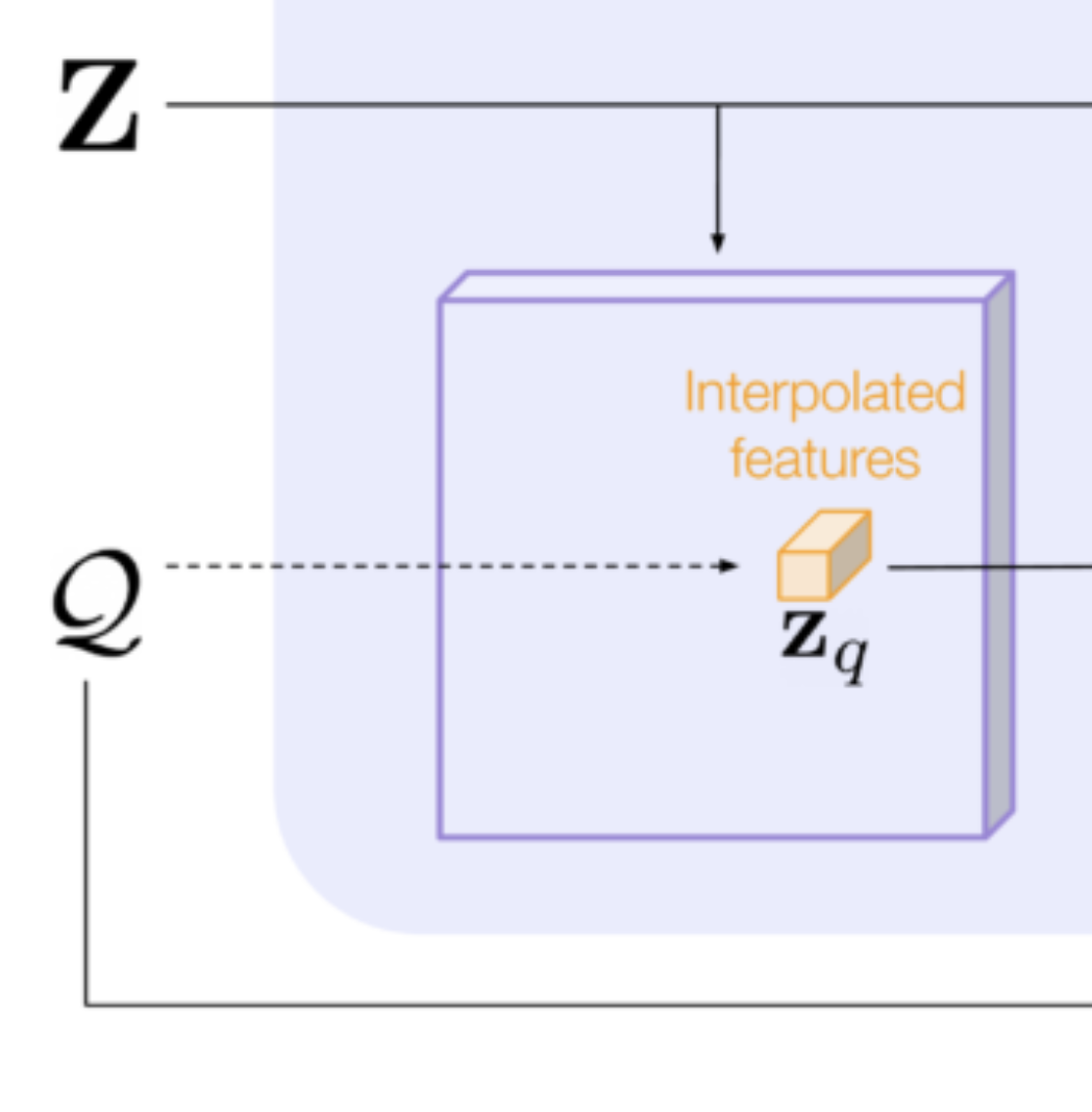
1. interpolates Z at the query location,
2. uses that interpolated feature vector to predict K attention offsets to other locations in the feature map,
3. interpolates Z at the offset locations for more feature vectors,
4. performs cross attention across all interpolated features to generate a final feature vector z, and
5. predicts occupancy and flow at each query point, using z.

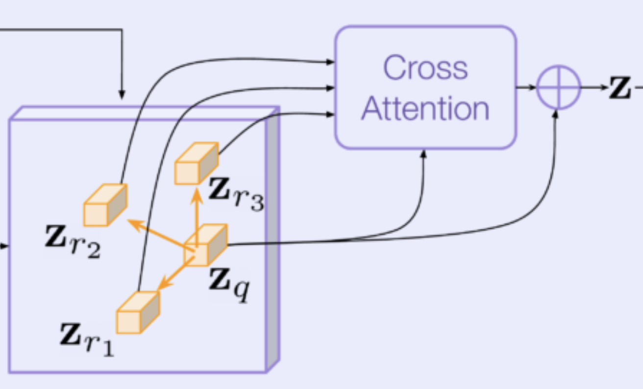
Local query feature vector $z_q\in {\mathbb{R}}^C$: The paper was motivated by the intuition that the occupancy at query point $q=(x,yt)\in \mathcal{Q}$ might be caused by a distant object moving at a fast speed prior to time $t$, so they wanted to use local features around the spatio-temporal query location to suggest where to look next (ex. looking back at the original position where the lidar evidence is or looking at neighboring vehicle locations). They used a combination of Deformable Convolution and Cross-attention.

They first extract local features from the feature map $\mathbf{Z}\in {\mathbb{R}}^{C\times \frac{H}{2}\times \frac{W}{2}}$. Given a query point $q_{x,y}=(x,y)$, they obtain a feature vector $z_q=\text{Interp}(\mathbf{Z},x,y)$ by bilinear interpolation. $(x,y)$ are continuous values so they need to use bilinear interpolation to extract a feature vector of $C$ channels from the surrounding grid cells since $(x,y)$ doesn’t necessarily fall in the center of a grid cell. $K$ reference points $\{r_1,\dots r_K\}$: You then predict $K$ reference points by offsetting the initial query point ${\mathbf{r}}_k=\mathbf{q}+\Delta {\mathbf{q}}_k$ where the offsets $\Delta \mathbf{q}$ are predicted using the network proposed in Convolutional Occupancy Networks.

Features for reference points ${\mathbf{z}}_{r_k}=\text{Interp}(\mathbf{Z},{\mathbf{r}}_k)$: You then obtain feature vectors for all of the reference points. 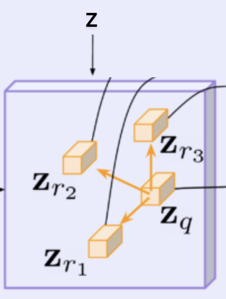This can be seen as a form of Deformable Convolution.

Cross-attention between local features and reference point features You then compute a learned linear projection of ${\mathbf{Z}}_q\in {\mathbb{R}}^{1\times C}$ and ${\mathbf{Z}}_r=\left\{{\mathbf{z}}_{r_1},\dots ,{\mathbf{z}}_{r_k}\right\}\in {\mathbb{R}}^{K\times C}$. Then, you compute cross-attention between the two projections to get a aggregated feature vector $\mathbf{z}\in {\mathbf{R}}^{1\times C}$ which contains information from both the local features and reference point features.

You then concatenate $\mathbf{z}$ and ${\mathbf{z}}_q$.

Predicting occupancy logits and flow for a query $q$ You then pass the concatenated $\mathbf{z}$ and ${\mathbf{z}}_q$ along with $q$, the $(x,y)$ location to a fully connected ResNet-based architecture with two linear heads (one for occupancy and one for flow).

Training §

Sample $|\mathcal{Q}|$ query points uniformly across the spatio-temporal volume $[0,H]\times [0,W]\times [0,T]$ where $H\in \mathbb{R},W\in \mathbb{R}$ are the height and width of a rectangular RoI in BEV surrounding the SDV (self-driving vehicle) and $T\in \mathbb{R}$ is the future horizon we are forecasting. You then pass the batch of query points with a single rendered lidar BEV and HD map to the model.

Loss §

They minimize the loss $\mathcal{L}={\mathcal{L}}_o+{\lambda }_{\mathbf{f}}{\mathcal{L}}_{\mathbf{f}}$ which is a linear combination of occupancy loss and flow loss.

Occupancy Loss Occupancy loss ${\mathcal{L}}_o$ is a binary Cross Entropy Loss between the predicted and ground truth occupancy at each query point $\mathbf{q}\in Q$. The predicted and ground truth occupancy values are in the range $[0,1]$. ${\mathcal{L}}_o=\frac{1}{|\mathcal{Q}|}{\sum }_{\mathbf{q}\in \mathcal{Q}}\mathcal{H}(o(\mathbf{q}),\hat{o}(\mathbf{q}))$ where $o(\mathbf{q})$ and $\hat{o}(\mathbf{q})$ are ground truth and predicted occupancies for query point $\mathbf{q}$.

The ground truth labels $o(\mathbf{q})$ are 1 if the query point lies within one of the bounding boxes of the scene and 0 otherwise.

Flow Loss The flow loss is only supervised for query points that belong to foreground (points that are occupied). This makes the model learn to predict the motion of a query location should it be occupied.

An L2 Loss is used where the ground truths are the backwards flow targets from $t$ to $t-1$ computed as rigid transformations between consecutive object box annotations. ${\mathcal{L}}_f=\frac{1}{|\mathcal{Q}|}{\sum }_{\mathbf{q}\in \mathcal{Q}}o(\mathbf{q})\Vert \mathbf{f}(\mathbf{q})-\hat{\mathbf{f}}(\mathbf{q}){\Vert }_2$

Results §

They evaluate the model using a regular spatio-temporal grid (even though during training they sampled randomly from a continuous space). They predict 5 seconds into the future with a resolution of 0.5 seconds.

In a slower speed dataset, AV2, they use a ROI around hero of 80x80 meters centered on hero at time $\bar{t}$ with a spatial grid resolution of 0.2 meters. In a highway dataset, HwySim, they use an asymmetric ROI with 200 meters ahead and 40 meters back and to the sides of hero at time $\bar{t}$ with a grid resolution of 0.4 meters. This is to allow handling fast vehicles moving up to 30 m/s in the direction of hero.

This is an interesting idea using different models depending on speed.