The following notes on object detection come mostly from EECS 498 Deep Learning for Computer Vision and EECS 442 Computer Vision at the University of Michigan.
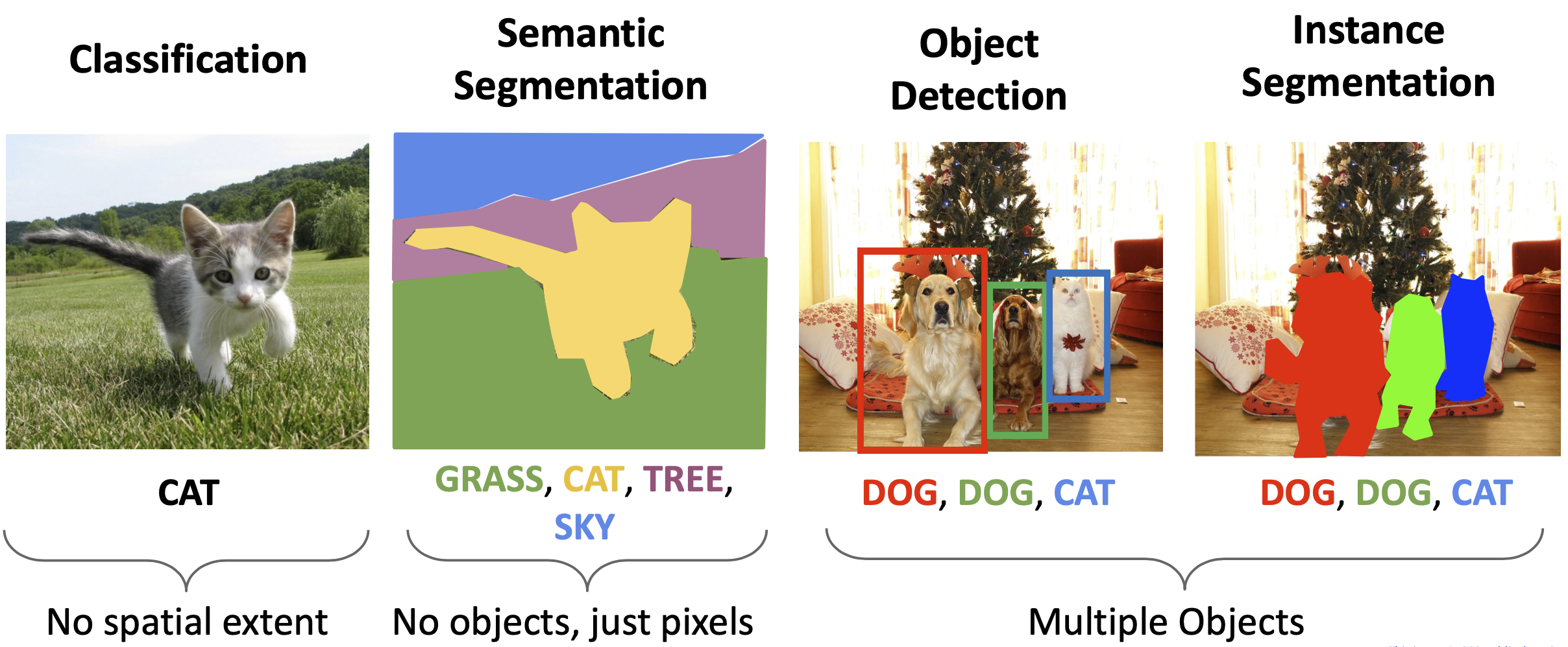
Previously in image classification, we’ve just assigned a single label to an entire picture. Now we want to get more fine-grained details. In scene understanding we saw we could give the most likely class for each pixel. However, now we want to say what each object is and give a bounding box for each object. This is a localization task (saying where something is in an image).
Each bounding box is defined by four numbers (x, y, width, and height). The boxes are aligned to the axis’s usually, so this is all the information you need.
The challenges in object detection are:
- We need to output a variable number of objects per image (not just the same number of class scores each time).
- We have multiple types of outputs: the label and the bounding box
- Large images: classification works at 224x224, but object detection needs higher resolution (~800x600). This is because we need enough resolution for each object we want to detect.
Bounding Boxes
Detecting a single object
A naive attempt at predicting bounding boxes would be to regress the bounding box (predict a single bounding box for an image). The model would have two branches: a “what” and a “where” branch.
- One branch gives class scores (and minimizes softmax loss)
- The other branch gives the bounding box coordinates (and minimizes the L2 difference from the correct coordinates).
- You combine the two losses with a weighted sum to get your total loss (you need a single scalar as the total loss for backprop to work). This type of problem is called a multitask loss.
- The feature extractor can be shared by both branches and can be pre-trained with transfer learning.
However, this is only able to output one bounding box for an entire image. This won’t work very well in practice.
Note: you could use IoU to calculate the loss for the bounding box, but if the bounding box has no overlap with the correct bounding box, then the IoU value will be 0. You want your grad function to have non-zero values for bad predictions.
Sliding Window
A slightly better (but not best) improvement is to use sliding windows. We can look at regions of the image and see if an object is contained in each region (similar to how we previously used a template of a chair in an image to look for chairs). The CNN will classify the crop as an object or background. However, we will also have to try different sized bounding boxes with different aspect ratios to capture differently sized objects. A 800x600 image has ~58 million boxes.
This was used predominantly before deep learning. It is very expensive to do this type of approach with models larger than a linear classifier since you need to check so many regions.
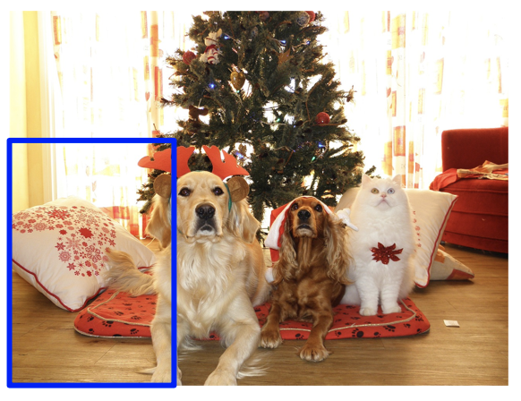
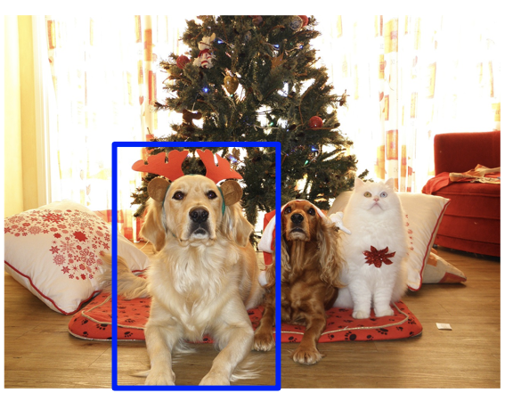 In the above example, we apply a sliding window to classify each region as background, dog, or cat.
R-CNN and Variants
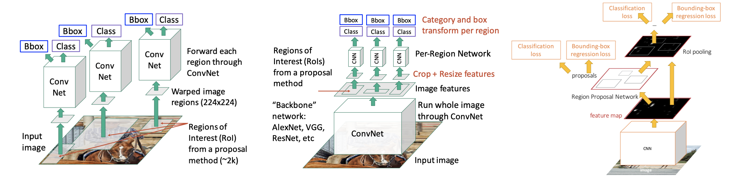 R-CNN: crop regions of interest generated by selective search (CPU) and then pass raw image features through a ConvNet.
Fast R-CNN: pass entire image through shared backbone. Run selective search (CPU) on the raw image, but crop features from the features output by the shared backbone. Then run a lightweight per-region network.
Faster R-CNN: pass entire image through shared backbone. Use a region proposal network (instead of selective search) (GPU) using the features output by the shared backbone as input. Then apply per-region network on the predicted regions using features output by the shared backbone.
R-CNN: crop regions of interest generated by selective search (CPU) and then pass raw image features through a ConvNet.
Fast R-CNN: pass entire image through shared backbone. Run selective search (CPU) on the raw image, but crop features from the features output by the shared backbone. Then run a lightweight per-region network.
Faster R-CNN: pass entire image through shared backbone. Use a region proposal network (instead of selective search) (GPU) using the features output by the shared backbone as input. Then apply per-region network on the predicted regions using features output by the shared backbone.
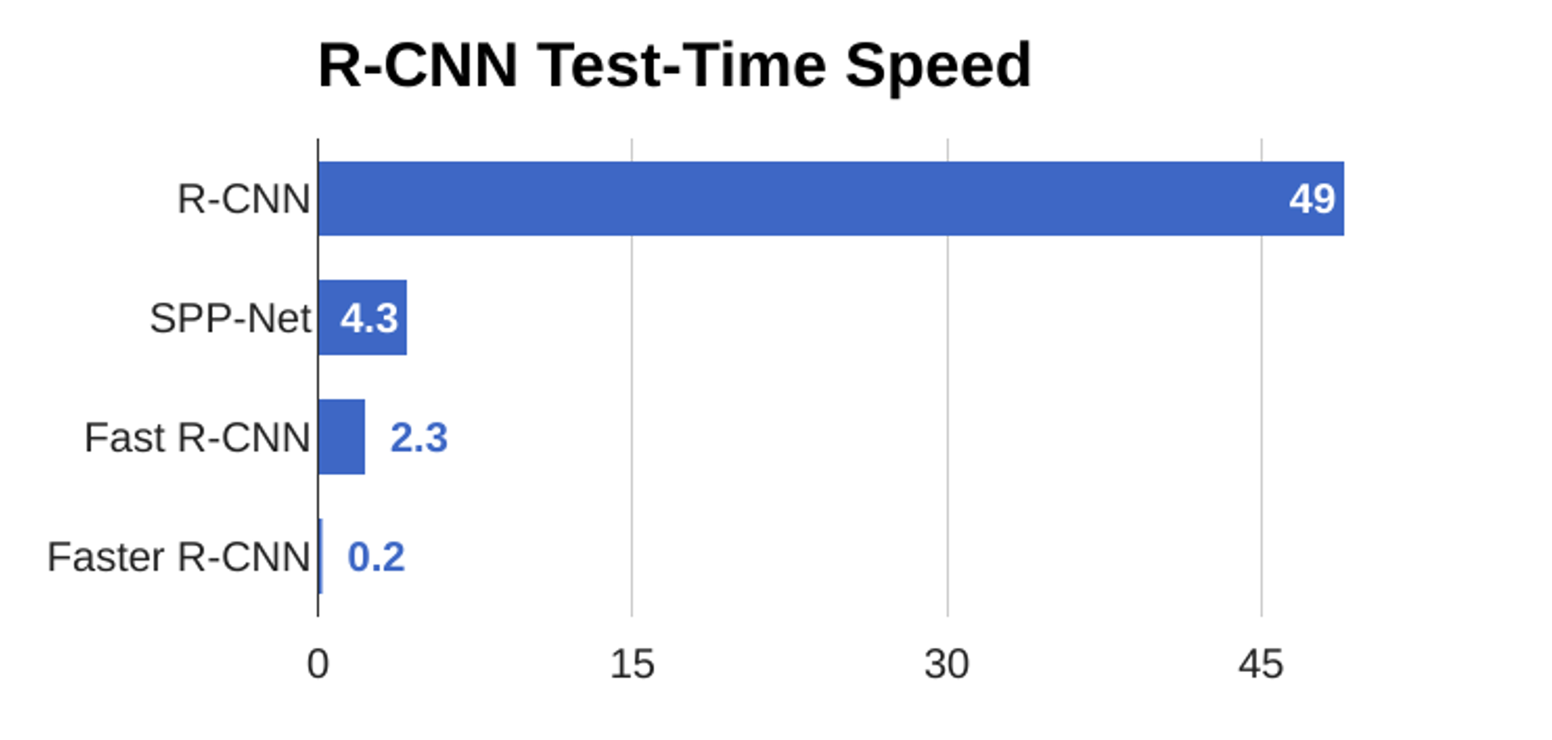 Time is shown in seconds.
Dealing with objects at different scales
Objects can appear in different sizes based on their location in the image (closer or further away). We want the object detector to be able to recognize objects regardless of their size.
Image Pyramid
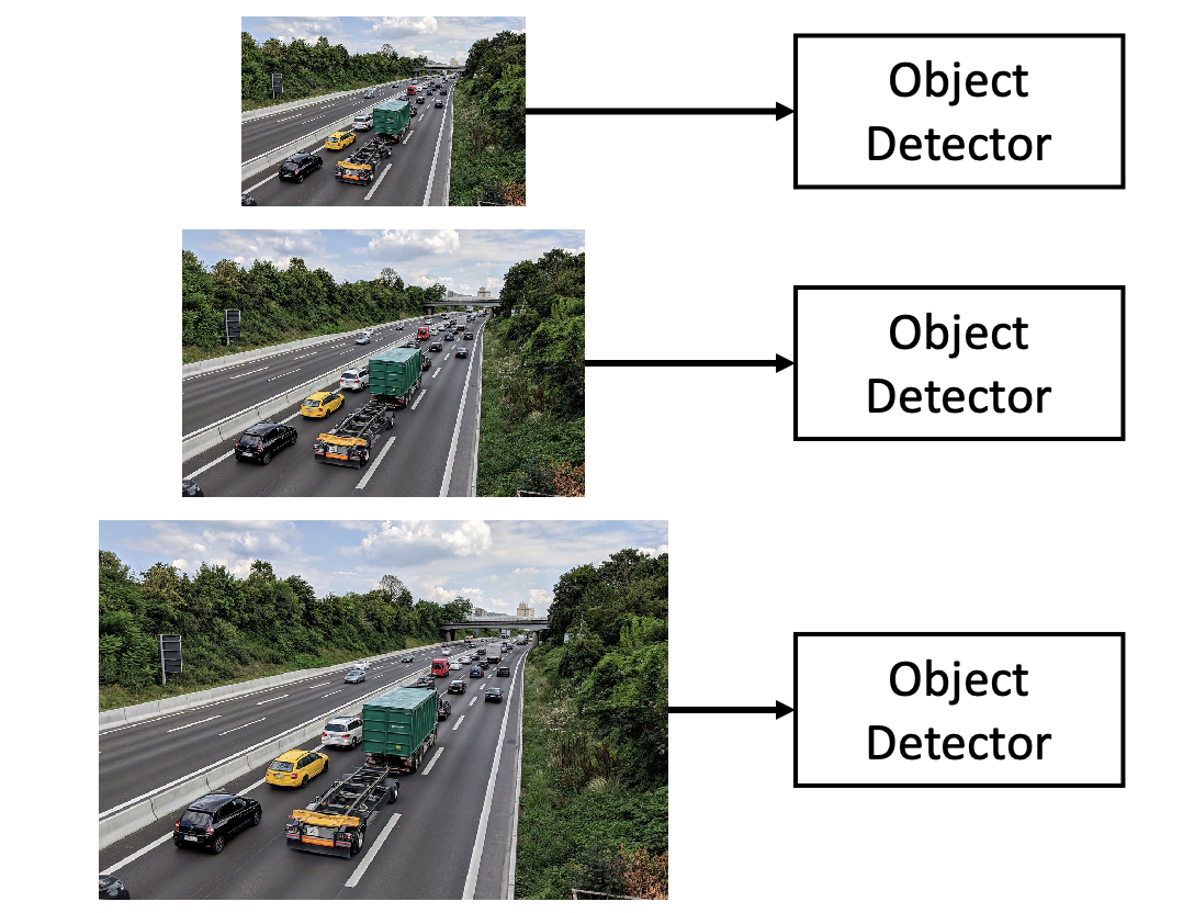
The classic idea is to build an image pyramid by resizing the image to different scales and processing each scale independently.
However, this is expensive because no computation is shared between the scales.
Multiscale Features
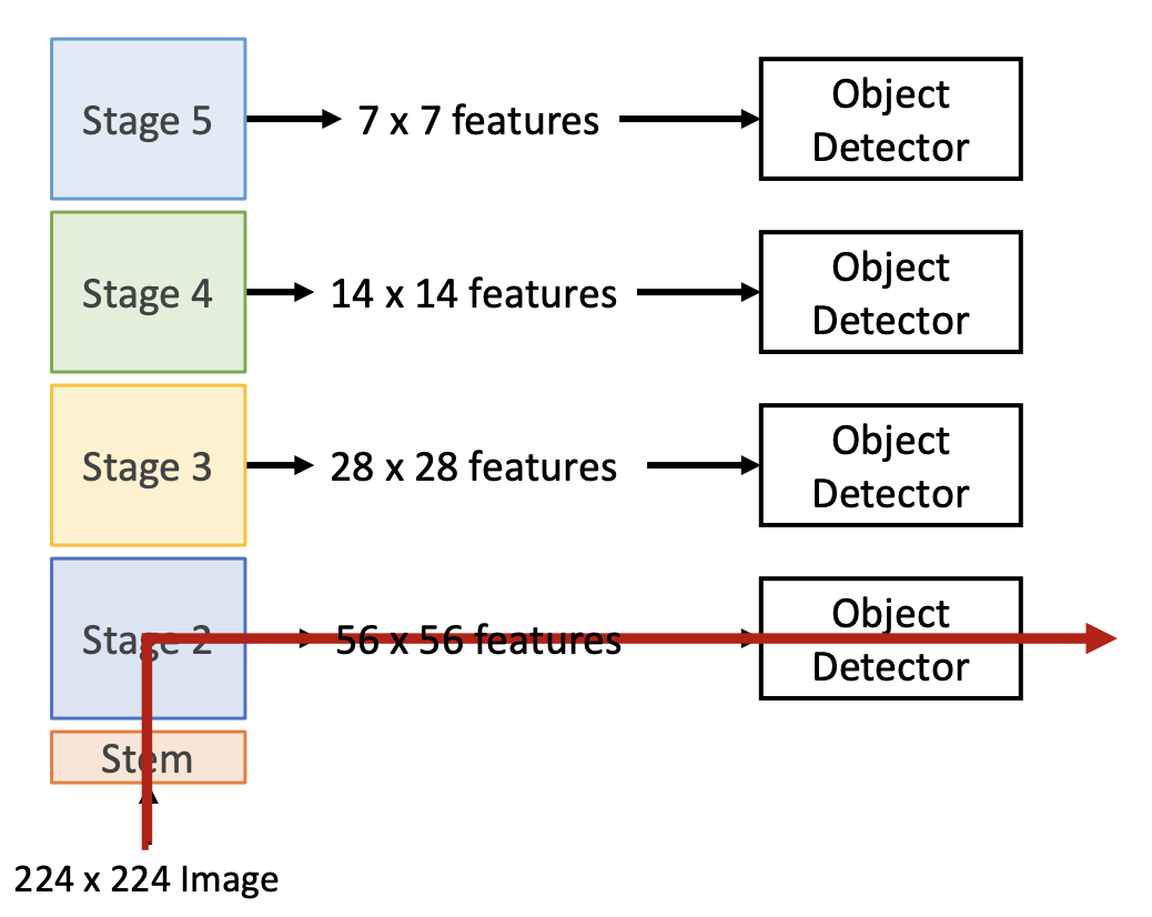 CNNs have multiple stages that operate at different resolutions. Each additional layer will be operating on an image of lower resolution (usually the spatial size of the layer decreases). You can attach an indepedent detector to the features at each level.
However, this has the problem that the detector on early features doesn’t make use of the entire backbone (shown in the red line above), so it doesn’t get access to high-level features. We can solve this problem using a Feature Pyramid Network.
One-shot detection (aka single-stage detectors)
R-CNN (and its variants) are considered a two-stage object detector. The first stage (run once per image) is the backbone network and region proposal network. The second stage (run once per region) is cropping, predicting the object class, and predicting bounding box offset.
One-stage detectors try to avoid needing the second stage and just generate predictions using the first stage. One-stage detectors process the image fully convolutionally and don’t have seperate networks that run on per-region features.
Single-Stage Detectors with Anchors
RetinaNet is one example of a single-stage detector. You take the raw image and run it through CONV layers to produce the bounding box outputs. It also makes use of anchor boxes. YOLO is another example (that also uses anchor boxes).
Single-Stage Detectors without Anchors
Working with anchors is annoying.
- Translation between bounding box coordinates in the feature map space and the image space.
- Lots of heuristics about matching ground truth bound boxes with the anchor bounding boxes.
- Extra hyperparameters: for each feature, you need to have a number of boxes, size, and aspect ratio.
Cross Stage Partial Networks: example of a network that doesn’t use anchors. FCOS - Fully Convolutional One Stage Object Detection: another anchor-free detector.
Evaluating an object detector
At test time, we predict bounding boxes, class labels, and confidence scores. We will compare these outputs with the ground-truth bounding box labels.
For every predicted bounding box we will have an IoU score. However, we don’t have a threshold for when to decide something is a good detection or not. We can use average precision for this. Average precision will give us a single number to decide how well our model performs based on precision (true positive / total detections) vs. our recall (true positive / total positive).
Mean average precision (mAP)
For image classification we were able to use accuracy as a metric to evaluate performance since we just had one label per bounding box. Now, however, we have multiple bounding boxes and multiple labels. We need a metric to quantify the overall performance of the model on a test set (so we can compare models).
Non-maximum Suppression
This is used to select high confidence and non-overlapping bounding boxes from the output of an object detection algorithm to use as the final predictions.