Swin v2

See: Swin Transformer.

What are the three main improvements of Swin v2 over Swin?

• Training instability is addressed with a residual-post-norm method combined with cosine attention to improve training stability.
• Resolution gaps between pre-training and fine-tuning (using models pre-trained on low-res images with high-res inputs) is addressed with a log-spaced continuous position bias method.
• Needing a large quantity of labelled data is addressed with a self-supervised method, SimMIM.

The paper trained a 3 billion-parameter Swin Transformer V2 model (largest dense vision model to date) and it can train with images up to 1,536x1,536 resolution.

Swin Transformer vs. Swin Transformer v2 §

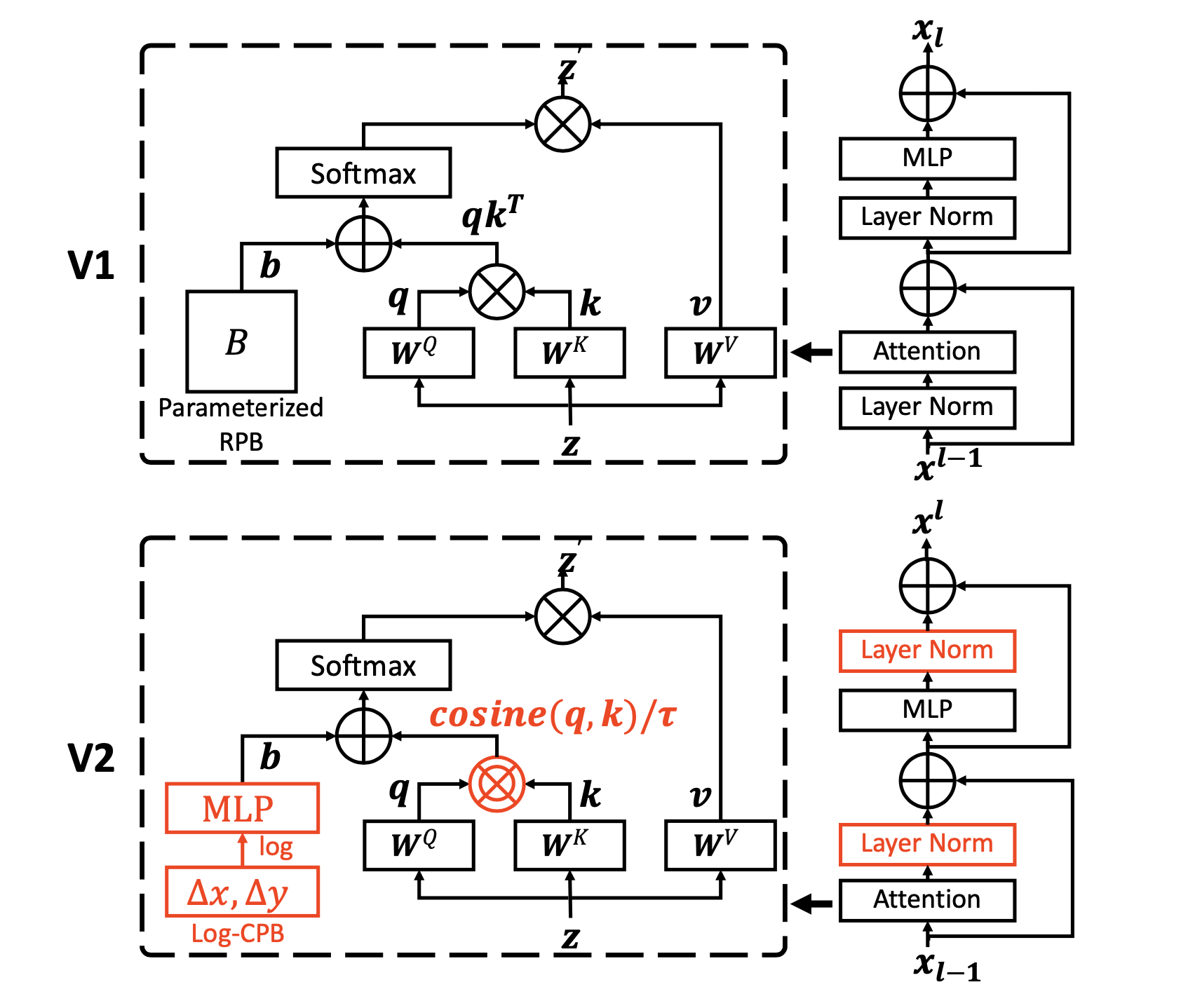
To better scale up model capacity and window resolution, several adaptions are made on the original Swin Transformer architecture (V1):

1. A res-post-norm to replace the previous pre-norm configuration (Layer Norm moved after Attention and MLP).
2. A scaled cosine attention to replace the original dot product attention.
3. A log-spaced continuous relative position bias approach to replace the previous parameterized approach (replaces the previous bias matrix $B$).

Adaptions 1) and 2) make it easier for the model to scale up capacity (training deeper models is more stable). Adaption 3) makes the model to be transferred more effectively across window resolutions. The adapted architecture is named Swin Transformer V2.

Residual post norm: §

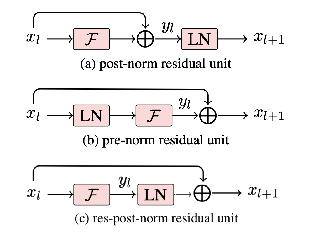
The original Attention is All You Need paper used post-norm:

x = norm(attn(x) + x)
x = norm(mlp(x) + x)

Swin Transformer, LayerScale, and ViT all use pre-norm

x = attn(norm(x)) + x
x = mlp(norm(x)) + x

Swin v2 uses res-post-norm:

x = norm(attn(x)) + x
x = norm(mlp(x)) + x

See Layernorm for a more thorough comparison.

Pre-norm results in activation amplitudes across layers becoming significantly greater in large models since the residual unit is directly added back to the main branch (attn(norm(x)) is non-normalized and updates the x value that will be propagated un-normalized due to the skip connections). This causes the activations to be accumulated layer by layer so the amplitudes at deeper lyers are significantly larger than those at early layers. For huge models, they were not able to complete training because the highest and lowest amplitudes were too large (magnitude of $10^4$).

The new approach results in the output of the residual branch being normalized before merging back into the main branch, so the amplitude of the main branch does not increase in later layers. Additionally, in the largest models, an additional layer normilization layer is added to the main branch every 6 Transformer blocks to increase stability. This additional layer was likely needed because although the outputs from the attn and norm layers are normalized, the value passed along by the residual connection will keep growing (ex. the first connection will pass x, the second will pass norm(attn(x)) + x, the third will pass norm(mlp(x)) + the previous value, etc.)

Scaled cosine attention to replace dot product attention §

• The scaled cosine attention makes the computation irrelevant to amplitudes of block inputs, and the attention values are less likely to fall into extremes.
• In the original Self-Attention Layer, the similarity terms of the pixel pairs are computed as a dot product of the query and key vectors. In large visual models, the learnt attention maps of some blocks and heads are frequently dominated by a few pixel pairs.

Swin v2 uses scaled cosine attention to compute the attention logit of a pixel pair $i$ and $j$ with: $\mathrm{Sim}\left({\mathbf{q}}_i,{\mathbf{k}}_j\right)=\cos \left({\mathbf{q}}_i,{\mathbf{k}}_j\right)/\tau +B_{ij}$ where $B_{ij}$ is the relative position bias between pixel $i$ and $j$, $\tau$ is a learnable scalar (not shared across heads and layers and set larger than 0.01). The cosine function is naturally normalized and therefore has milder attention values.

Language Models vs. Vision Models §

• Transformer-based language models have been able to scale very well and have found to possess increasingly strong few-shot capabilities akin to human intelligence for a broad range of tasks.
• Language modeling has been encouraged by the discovering of a scaling law (Scaling Laws for Neural Language Models).
• The scaling up of vision models has lagged behind. Larger vision models usually perform better, but there size has been limited and the largest models are usually just used for image classification. The paper claims this is “due to inductive biases in the CNN architecture limiting modeling power.”

Instability in training §

• The discrepancy of activation amplitudes across layers becomes significantly greater in larger models.
• This is caused by the output of the residual unit being directly added back to the main branch. The result is that the activation values are accumulated layer by layer, and the amplitudes at deeper layers are thus significantly larger than those at early layers.
• To address this, they propose a new normalization configuration called res-post-norm which moves the LN layer from the beginning of each residual unit to the back-end. This new activation produces much milder activation values across the network layers.
• They also propose a scaled cosine attention to replace the previous dot product attention. This makes the computation irrelevant to amplitudes of block inputs, and the attention values are less likely to fall into extremes.

Working with high resolution inputs §

Log-spaced continious position bias §

Problem: many downstream vision tasks require higher resolution input images or large attention windows. If the model is trained on low-resolution images, then the window size variations between the low-resolution pre-training and high-resolution fine-tuning can be quite large.

• Global vision transformers (like ViT) will increase the attention window size linearly proportional to the increased input image resolution (ex. if the image width doubles, each attention window will double in width and the number of patches remains the same). For local vision transformer architectures (like swin), the window size can be either fixed or changed during fine-tuning. Allowing varying window sizes is more convenient because the window size can be divisible by the entire feature map size and you can tune receptive fields for better accuracy.
• The current approach to handling varying window sizes between pre-training and fine-tuning is to perform a bi-cubic interpolation of the position bias map.

Swin V2’s solution to window size variations

• This paper introduces a log-spaced continious position bias (Log-CPB) which generates bias values for arbitrary coordinate ranges by applying a small meta network on the log-spaced coordinate inputs.
• The meta network takes the log of the difference between any pair coordinates, so a pre-trained model will be able to freely transfer across window sizes by sharing weights of the meta network. This allows you to use different window sizes and different window grid configurations depending on the images you want to work on (ex. $3\times 4$ grid or $4\times 4$ patch).
• A critical design of Swin V2’s approach is to transform the coordinates into the log-space so that the extrapolation ratio can be low even when the target window size is significantly larger than that of pre-training.

Position bias meta network Instead of directly optimizing the parameterized biases (ex. using $\hat{B}\in {\mathbb{R}}^{(2M-1)\times (2M-1)}$ like Swin), Swin V2 uses a small network on the relative coordinates: $B(\Delta x,\Delta y)=\mathcal{G}(\Delta x,\Delta y)$

Where $\mathcal{G}$ is a small network (ex. a 2-layer MLP with a ReLU activation in between by default).

The meta network $\mathcal{G}$ generates bias values for arbitrary relative coordinates and can be transferred to fine-tuning tasks with varying window sizes (you can fine-tune $\mathcal{G}$). In inference, the bias values at each relative position can be pre-computed and stored as model parameters so the inference is the same as the original parameterized bias approach.

Log-spaced coordinates Swin V2 calculates the relative coordinates using log-spaced vs. linear-spaced coordinates:

$\begin{array}{rl}& \widehat{\Delta x}=\mathrm{sign}(x)\cdot \log (1+|\Delta x|)\\ & \widehat{\Delta y}=\mathrm{sign}(y)\cdot \log (1+|\Delta y|)\end{array}$

Note: you use the magnitude of the coordinate difference inside the log since the log of a negative number is undefined. You then multiply by the sign of the difference to preserve positive/negative information.

• When transferring across varying window sizes, a large portion of the relative coordinate range needs to be extrapolated.
• Using log-spaced coordinates allows the required extrapolation ratio to be smaller than when using the original linear-spaced coordinates.
• The log-spaced CPB approach performs best, particularly when transfered to larger window sizes.

With the log-spaced coordinates, transferring from a pre-trained 8x8 window size to a 16x16 window size, the extrapolation window will be 0.33x the original ratio

Using the original window size, the input coordinate range will be from $[-7,7]\times [-7,7]$ to $[-15,15]\times [-15,15]$. The extrapolation ratio is $\frac{8}{7}=1.14\times$ of the original range.

Using the log-spaced coordinates the input range will be from $[-2.079,2.079]\times [-2.079,2.079]$ to $[-2.773,2.773]\times [-2.773,2.773]$. The extrapolation ratio is 0.33× of the original range, which is an about 4 times smaller extrapolation ratio than that using the original linear-spaced coordinates.

Dealing with larger GPU memory consumption §

• Scaling up of model capacity and resolution results in large GPU memory consumption.
• To solve this issue, the paper uses zero-optimizer, activation check pointing, and a new implementation of sequential self-attention computation to reduce memory consumption with a marginal effect on training speed.

Zero Optimizer

• In a general data-parallel implementation of optimizers, the model parameters and optimization states are broadcasted to every GPU. This implementation is very unfriendly on GPU memory consumption.
• With a ZeRO optimizer, the model parameters and the corresponding optimization states will be split and distributed to multiple GPUs, which significantly reduces memory consumption.
• We adopt the DeepSpeed framework and use the ZeRO stage-1 option in our experiments. This optimization has little effect on training speed.

Activation Checkpointing (Training deep nets with sublinear memory cost):

• Feature maps in the Transformer layers also consume a lot of GPU memory, which can create bottlenecks when image and window resolutions are high.
• The activation checkpointing technology can significantly reduce the memory consumption, while the training speed is up to 30% slower.

Sequential self-attention

• Implement self-attention sequentially instead of using the more common batch computation approach.
• This is applied to the first two stages (which have more windows and larger feature maps) and has little impact on the overall training speed.

Reducing need for large labelled datasets §

• They used Self-supervised Learning to pre-train without tons of labeled data (40x less labelled data than in JFT-3B).
• Specifically, they use SimMIM.

Results §

• The shrunken gains by SwinV2-L than that of SwinV2-B may imply that if ex- ceeding this size, more labeled data, stronger regularization, or advanced self-supervised learning methods are required.
• Suggests that scaling up vision mod- els also benefits video recognition tasks.
• Res-post-norm and scaled cosine attention are more beneficial for larger models. They also stabilize training.
• The larger the changes in resolution between pre-training and fine-tuning, the larger the benefit of the proposed log-spaced CPB approach.