Multi-Agent Motion Forecasting as Language Modeling

The following are my personal notes on the paper MotionLM.

This paper achieves #1 on Waymo Open Motion Dataset (2023) by formulating multi-agent motion prediction as a language modeling task. They liken road agents to participants in a dialogue who exchange a dynamic series of actions and reactions and represent continuous trajectories as sequences of discrete motion tokens.

The main contributions of the work are:

1. Model multi-agent motion forecasting as a language modeling task and decode the motion tokens respecting temporal causality (previous behavior affects later behavior).
2. They combine sampling from the model with a weighted mode identification (identifying the most likely trajectory) to identify the most likely trajectories.

The model does not require anchors or explicit latent variable optimization to learn multimodal distributions.

Anchors are (often) heuristically defined points that an agent trajectory may pass through/terminate. Using anchors allows predicting a probability distribution over a fixed set of points vs. a continuous 2D plane. See TNT for an example of one paper that uses anchors.

Explicit latent variable optimization means that your latent (hidden) dimension is optimized over. An example of this is the paper PRECOG (PREdiction Conditioned On Goals in Visual Multi-Agent Settings) which samples from a latent variable $\mathbb{Z}$ (a simple distribution like a normal distribution) and then predicts scenes.

Related Work §

Marginal vs. Joint Prediction §

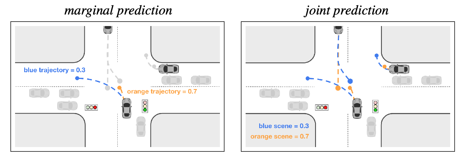
Joint probability is the probability of two events occurring simultaneously. Marginal probability is the probability of an event irrespective of the outcome of another variable. Marginal agent predictions may conflict with each other (have overlaps), while consistent joint predictions should have predictions where agents respect each other’s behaviors (avoid overlaps) within the same future.

Left: Marginal prediction for bottom center vehicle. Scores indicate likelihood of trajectory. Note that the prediction is independent of other vehicle trajectories. Right: Joint prediction for three vehicles of interest. Scores indicate likelihood of entire scene consisting of trajectories of all three vehicles.

Link to original

Marginal models §

Marginal models predict independent per-agent distributions of likely behavior. These are insufficient as inputs to a planning system because they do not represent the future dependencies between the actions of different agents which causes inconsistent scene-level forecasting (two agents may independently have a high probability of merging into a lane but it’s unlikely both will merge into the same lane).

Joint models that don’t respect temporal dependencies §

Some models first generate marginal trajectories (independent for each agent) and then merge the trajectories through a learned or heuristic method.

However, these approaches do not model temporal dependencies within trajectories so when combining independent trajectories they may be susceptible to capturing spurious correlations (ex. they can capture the correlation between a lead and decelerating and a trailing one decelerating but not be able to infer which one is causing the other to slow down) which can lead to poor predictions.

Joint models that respect temporal dependencies §

Existing models that produce joint trajectories (consider agent interactions with each other) have usually relied on explicit latent variables for diversity (ex. you don’t always want to predict that the tailing agent will always patiently follow the lead agent) which is optimized via an evidence lower bound (GANs) or Normalizing Flows.

Using explicit latent variables means you are representing the sample space of all points via a distribution and then you are able to sample from this distribution in order to get diversity in your samples.

GANs do this by having a generator that starts with random noise (sampled from a simple distribution) and then using a generator to produce a scene. It is trained by using a discriminator who says whether the scene is likely real or not.

Normalizing Flows do this by learning an invertible mapping from the original scene to a point in a distribution where you want the mapped points corresponding to the examples in your dataset to have high probability. You can then invert the learned function, sample a point from your distribution, and then use the inverted function to produce a scene.

MotionLM §

• They maximize the average log probability over sequence tokens.
• They don’t need heuristics to merge individual agent trajectories and instead directly produce joint distributions over interactive agent futures.
• At inference time, joint trajectories are produced step-by-step and agent sample tokens simultaneously attend to one another at each step. The temporal rollout makes the trajectories temporally causal (previous behavior affects future behavior but not vice-versa) and attending to other agent tokens makes the predictions joint. Being temporally causal allows conditional forecasting.
• Previous approaches forced trajectory multimodality during training (ex. predicting probabilities for the agent going left, straight, and right). MotionLM is latent variable and anchor free and multimodality (getting different trajectories) comes from sampling.
• MotionLM can be applied to marginal, joint, and conditional predictions.
• They discretize the continuous 2D plane into uniform axis-aligned deltas between consecutive waypoints of agent trajectories.
• They represent agent trajectories as waypoints that are binned axis-aligned deltas from the previous waypoint (how far you move along the x and y axis from the previous waypoint). The binning of the deltas makes this a classification problem instead of a regression problem.

Joint probabilistic rollouts §

They sample a predicted action for each target agent at each future timestep. The target action for the $n$th agent at time $t$ is represented as $a_t^n$ and the set of actions for all agents at time $t$ is represented as $A_t\doteq \left\{a_t^1,a_t^2,\dots ,a_t^N\right\}$.

Factorization §

They factorize the probability of all actions for all agents across all future steps dependent on scene features as the following product of conditionals:

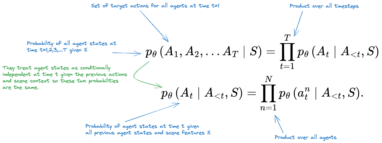
They treat agent actions as conditionally independent at time $t$ given the previous actions given the previous actions and scene context ($A_t$ depends only on $A_{<t}$ and $S$). Therefore, $p_{\theta }(A_1,A_2,\dots A_T\mid S)$ (the probability of the agent states at all time steps given the scene features) is equivalent to $p_{\theta }(A_t\mid A_{<t},S)$ (the probability of the agent state at time $t$ given the previous agent states and scene features).

They treat agent actions as independent at the time step being currently rolled out because human drivers generally require at least 500 ms to react. Therefore what another agent is doing at the exact same time will not cause an immediate change in another agents current behavior.

Training objective §

MotionLM is a generative model trained to match the joint distribution of agent behavior in the training dataset (probability of all agent actions occurring at each timestep given scene features).

They attempt to maximize the likelihood of $A_t$ given the previous agent actions $A_{<t}$ and the scene features $S$: $\arg {\max }_{\theta }{\prod }_{t=1}^T{p}_{\theta }(A_t\mid A_{<t},S)$ They use Teacher Forcing where the previous ground truth (not predicted) tokens are provided at each timestep. This allows for parallelization across time when training since you aren’t dependent on the previous steps predictions.

MotionLM Architecture §

They have two main networks:

• An encoder to process scene elements.
• A decoder to perform cross-attention to the scene encodings and self-attention along agent motion tokens.

We first encode heterogeneous scene features relative to each modeled agent (left) as scene embeddings of shape $R,N,\cdot ,H$. Here, $R$ refers to the number of rollouts, N refers to the number of (jointly modeled) agents, and H is the dimensionality of each embedding. We repeat the embeddings $R$ times in the batch dimension for parallel sampling during inference. Next, a trajectory decoder autoregressively rolls out $T$ discrete motion tokens for multiple agents in a temporally causal manner (center). Finally, representative modes of the rollouts may be recovered via a simple aggregation utilizing k-means clustering initialized with non-maximum suppression (right).

Scene Encoder §

$S$ represents the input data for a given scenario (roadgraph elements, traffic light states, road agent features and recent histories, etc.). The goal is to generate joint agent states $Y_t=\left\{y_t^1,y_t^2,\dots ,y_t^N\right\}$ for $N$ agents of interest at future timesteps $t=1,\dots ,T$. The future state targets are two-dimensional waypoints $(x,y$) coordinates with $T$ waypoints forming the full ground truth trajectory for an agent.

The features are extracted with respect to each modeled agent’s frame of reference. The encoder then consists of self-attention layers that exchange information across all past timesteps and agents.

In the first layer of the decoder, latent queries (a fixed number of queries that the model learns the contents of) are used to cross-attend to the original inputs in order to reduce the number of vectors being processed from the number of scene features to just the fixed number of latent queries.

Joint trajectory decoder §

They represent the trajectories of continuous waypoints into sequences of discrete tokens to allow treating prediction as a classification task vs. a regression task.

The trajectory decoder is implemented via a transformer that takes in the motion tokens (all agents at all times) as queries and the scene encodings as context. It first performs cross-attention between the motion tokens and the scene encodings and then performs self-attention along the motion tokens.

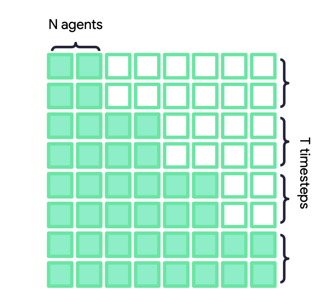
They use masked casual attention during training so the agents can attend to each other’s previous motion tokens (solid squares) but no future tokens (empty squares).

Quantization:

Quantization approach

They represent trajectories as a series of $T$ waypoints that they then discretize into delta bins for change in $(x,y)$ location with 128 bins per axis. They then use a “Verlet” wrapper to reduce the number of bins per axis to 13. They then take the Cartesian product of the sets of possible bin indices in each direction to form a vocabulary of ($13\cdot 13=169$ tokens) that they can index into with a single integer prediction.

To extract the discrete ground truth trajectory tokens, they first normalized each agent’s ground truth trajectory with respect to the position and heading of the agent at time $t=0$.

They create delta actions between each waypoint using a uniformly quantized $(\Delta x,\Delta y)$ vocabulary formed by a total number of per-coordinate bins and a max/min delta value. The paper used a delta interval from [-18 m, 18 m] and 128 bins.

You can therefore map a single-coordinate (x or y) delta action to one of the bins (x or y respectively) and you can represent each action delta as a single $(\Delta x,\Delta y)$ action per step.

They then collapse the per-coordinate actions to a single integer indexing into the bins Cartesian product.

Cartesian Product

The Cartesian product A × B of sets A and B is the set of all possible ordered pairs with the first element from A and the second element from B. For example, if $A=\{a1,a2\}$ and $B=\{b1,b2\}$, the Cartesian product $A\times B=\{\{a1,b1\},\{a1,b2\},\{a2,b1\},\{a2,b2\}\}$.

Mapping into the Cartesian product between the possible delta actions for the x and y axises allows using a single index instead of needing two for each axis. They use 13 tokens per-coordinate (after the Verlet wrapper is applied) which results in $13^2=169$ total discrete tokens available in the vocabulary (169 elements in the Cartesian product).

Embedding They have a learned value embedding and two learned positional embeddings (one for timestep and one for agent identity) for each discrete motion token. These embeddings are combined via an element-wise sum prior to being input to the decoder.

This is saying you have three weight matrices: $W_v,W_t,W_a$

• $W_v$ is an embedding for the motion token information
• $W_t$ is an embedding for the timestep $t$ that the token lies within a full trajectory
• $W_a$ is an embedding for agent information You then do: $W_v(\text{token})+W_t(\text{timestep})+W_a(\text{agent})$ with an element-wise summation.

Flattened agent-time self-attention: They perform self-attention in the decoder over the flattened sequences of all agents’ ($N$ agents) motion tokens over time ($T$ time). This means they perform attention over $NT$ tokens which is $(NT{)}^2$ complexity since each token attends to all other tokens.

This has the downside that as the number of agents in the scene grows, you have to do a lot more computation. However, the number of agents in most scenes considered is very small (WOMD only predicts 2 agents at 8 seconds each at 2 Hz. This requires 16 time steps for 2 agents which is 32 tokens).

You could alternatively do separate passes for agents and time ($N$ followed by $T$ vs. $NT$).

Ego agent reference frames: The decoder also performs cross-attention between the agent motion tokens and the agent-centric feature encodings. The scene features are extracted with respect to a particular agent, so they split up the $NT$ sequence into a batch of length $N$ with $T$ tokens in each example of the batch.

They then compute cross-attention for each of the $N$ agents between its $T$ motion tokens and the scene features that were extracted with respect to it. This treats each modeled agent as if it were the “ego” agent once (the scene is with respect to it) and moving the ego agents into the batch dimension allows parallelization during training and inference.

Manipulating Predictions §

The default behavior of the decoder looks like the following network which is called a Causal Bayesian Network for joint rollouts. You roll out each timestep $t$ and the action of all agents (ex. $x,y$) depends on the actions of all other agents (and itself) at all previous time steps. You can see at $t=2$ that $y$ is affected by $x=1,y=1$ (but not $x=2$ since you don’t attend to other agents at the same timestep).

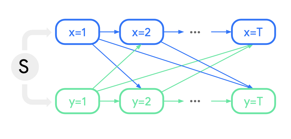
Causal interventions can only be approximated by the model

The paper states that cause/affect relationships can’t be learned from observational data in general since you can have unobserved confounders.

(In causal inference, a confounder is a variable that influences both the dependent variable and independent variable, causing a spurious association.)

However, the model’s factorization (looking only at previous time steps) allows it to break spurious correlations that could come from not respecting temporal causality (a future action impacting a previous one).

Post-intervention Bayesian network §

They can query for “temporally causal conditional rollouts” by fixing a query agent to take some sequence of actions and only rolling out the other agents (but still only looking at previous agent behavior). This lets you do things like “if hero drives this way, what will the other agents do?” As expected, temporally causal conditional rollouts result in more accurate predictions for the target agent by fixing what one agent will do.

An example of the difference in behavior is shown below. When the pedestrian is considered independently (marginal), the model predicts it will cross the road. When the model is conditioned on the vehicle’s GT turn (magenta), the pedestrian is instead predicted to yield. ![[Research-Papers/multi-agent-motion-forecasting-as-language-modeling-srcs/screenshot 2023-11-25_17_01_25@2x.png]]

Acausal conditoning §

You can also allow the actions of one agent to be viewed in the future by other agents (violating causal conditioning). This means that if you condition on agent $x=i$, it will affect all agents $y=j$ for $i\ge j$ for all time steps. 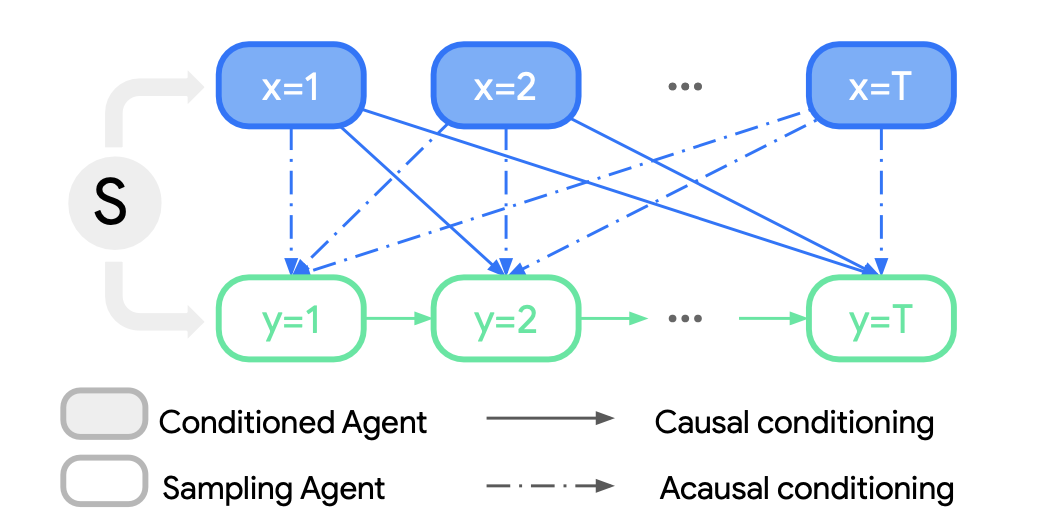This means if you had agents $\{1,2,3\}$ and conditioned on agent 2, agent 1 would be unaffected ($2\nleqq 1$) but agent $3$ would see all of agent 2’s behavior.

Acausal conditioning results in even more accurate results than temporally causal conditioning. However, the improvements are largely due to predictions that wouldn’t make sense if they were interpreted as predicted reactions to the query agent.

You need to be careful when evaluating performance using acausal conditioning

If you leak what the autonomous vehicle is going to do to the model, then it will make predictions for other agents that match the AV’s behavior.

For instance, if you have an AV trailing another agent but leak that the AV will continue moving forward, then the model will likely predict the lead agent will also move forward even though it is really the lead agent moving forward that would cause the AV to move forward.

Rollout Aggregation §

Joint motion prediction benchmarks like WOMD require predicting a small number of future “modes” where each mode corresponds to a specific homotopic outcome (ex. pass/yield).

They aggregate the rollouts to find the different modes and assign a probability to each mode.

The aggregation is done using an NMS aggregation scheme similar to the one used by MultiPath ++.

They also use model ensembling to reduce epistemic uncertainty (differences in model output that vary from one trained model to another) and combine rollouts from independently trained models prior to the aggregation step. They use 8 independently trained models that each generate 512 rollouts.