BEVFusion

This paper proposes a new sensor fusion framework that combines multi-modal features in a BEV (bird’s eye view) representation space. This preserves both geometric (from lidar) and semantic (from camera) information and is a space friendly to almost all perception tasks since the output space is usually also BEV. The approach can be used for a variety of 3D perception tasks.

Introduction §

Cameras capture data in perspective view and lidar in 3D view. Existing approaches for merging the two either involve projecting lidar points onto a 2D image and processing the RGB-D data with 2D CNNs or adding image features point-wise to the lidar point cloud (aka point wise fusion) which was previously the best approach.

You need to use a fusion approach vs. just encoding each sensor individually and performing a naive elementwise feature fusion won’t work since the same element in different feature tensors might correspond to different spatial locations. Therefore, you need a shared representation such that all sensor features can easily be converted to it without information loss and it is suitable for different types of tasks.

Projecting lidar points onto a 2D image:

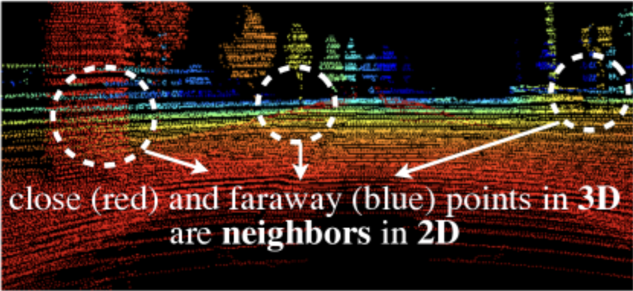
Projecting lidar points onto a 2D image results in losing geometric information (points that are far away from each other can appear closer when projecting into 2D).

Projecting image features onto a point cloud

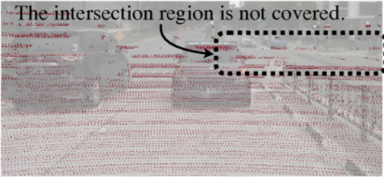
The camera-to-lidar projection is semantically lossy since for a typical 32-beam lidar only 5% of camera features will be matched to a lidar point and all other pixel features will be dropped.

Related Work §

They mention various works that focus on:

• Lidar only 3D perception
• Camera only 3D perception
• Multi-sensor fusion approaches which either use proposal-level or point-level.
  • Proposal-level predicts a 3D region for the point cloud and then extract image features for that RoI. This approach is object-centric and can’t work for things like BEV map segmentation where you don’t have a predicted RoI. (ex. TransFusion)
  • Point-level will add image semantic features onto foreground lidar points and perform lidar based detection.
• Multi-task learning approaches have trained a model to simultaneously perform multiple tasks (ex. object detection and instance segmentation) but these have not considered multi-sensor fusion.

Method §

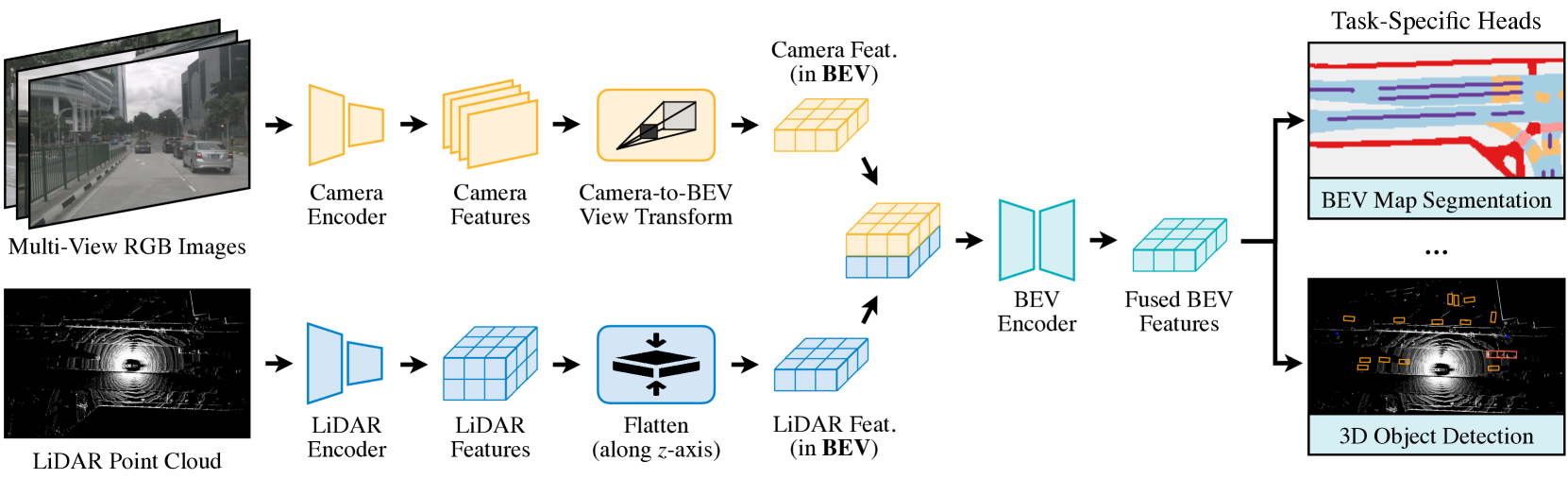They first use modality-specific encoders to extract features independently from the different sensors. They then transform the multi-modal features into a unified BEV representation using an optimized kernel.

They then apply the convolution-based BEV encoder to the unified BEV features to alleviate the local misalignment between different features (aka the BEV features from different sensors don’t line up perfectly spatially). Finally, they append a few task-specific heads to support different 3D tasks.

Camera to BEV Transformation §

The camera to BEV transformation consists of first projecting the camera to a 3D point cloud and then converting the 3D point cloud to a 2D BEV feature.

Camera to 3D point cloud

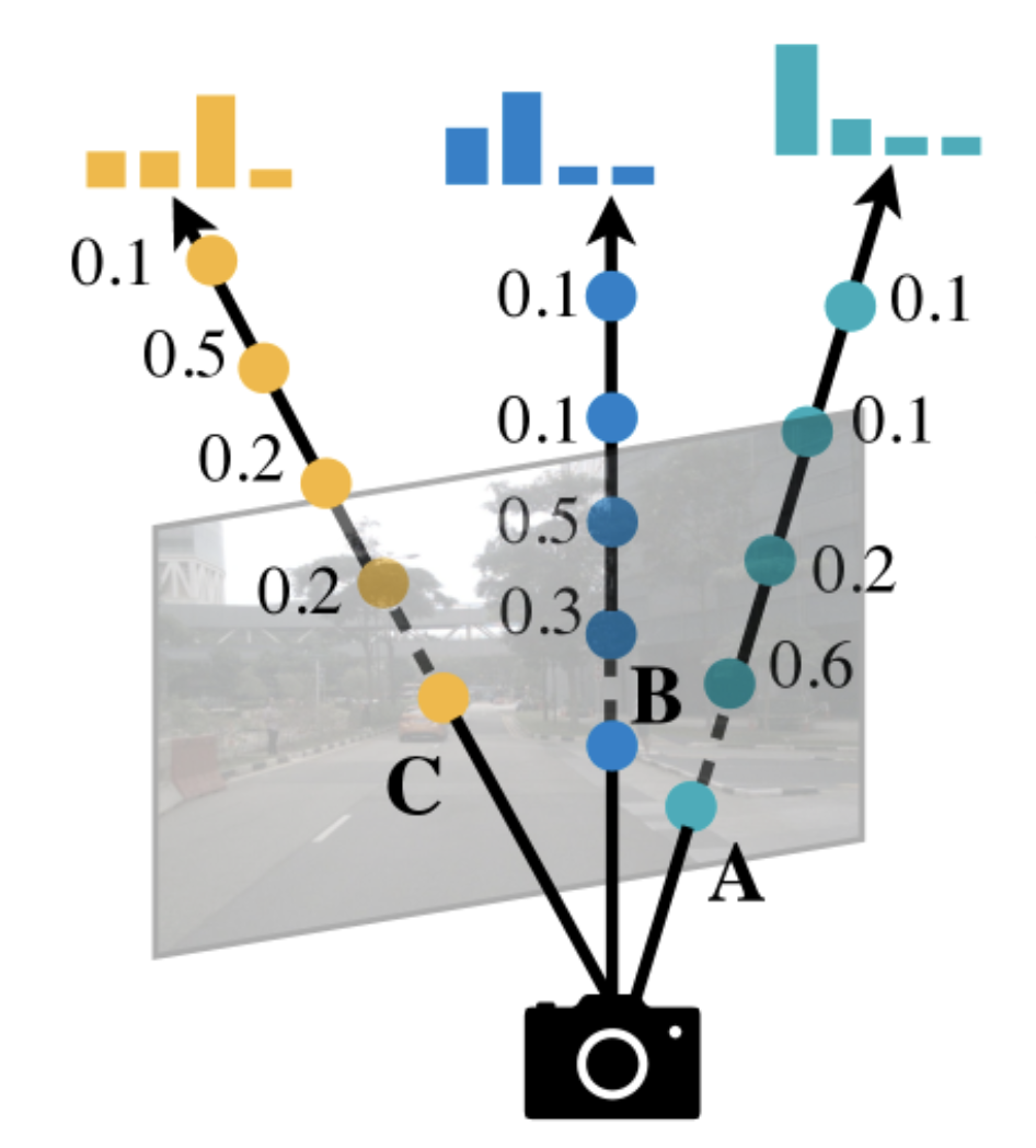
The camera-to-BEV transformation is difficult because the depth associated with each camera feature is ambiguous. The paper predicts a discrete depth distribution for each pixel. You then scatter each feature pixel into $D$ discrete points along the camera ray and rescales the associated features by their corresponding depth probabilities. This gives you a camera feature point cloud of size $NHWD$ where $N$ is the number of cameras and $(H,W)$ is the camera feature map size.

Camera-to-BEV TLDR

You have a height, width, depth grid of dims $(H,W,D)$ and for each pixel’s features in the original $(H,W)$ image you project that pixels feature along the camera’s ray.

Note you aren’t just repeating the same (H, W) feature map at different depths since the camera rays don’t just go straight back.

See Lift, Splat, Shoot for more details on the projection.

Converting the 3D camera point cloud into BEV The 3D camera feature point cloud is quantized along the $(x,y)$ axis with a step size of $r$ (ex. 0.4 meters). This divides the $(x,y)$ plane into a grid of $(x/r,y/r)$ cells.

For each $r\times r$ BEV cell you then perform BEV pooling to aggregate the features and then flatten the features along the z-axis.

The BEV pooling operation is very slow since the camera feature point cloud is very large. There could be around 2 million points generated for each frame (two orders magnitudes denser than a lidar feature point cloud).

Precomputation When you project the image into 3D you will end up with a $NHWD$ point cloud. This point cloud is not a dense grid since each pixel projects along a different ray and not all space will be filled. Instead, it is just a list of $NHW$ pixels ($N$ cameras) where each pixel has a corresponding distribution along $D$ bins.

You then need to take this list of points and use the camera intrinsics and extrinsic to determine how the pixels will project along camera rays and where they will end up in 3D space. Unlike lidar points whose 3D location depends on what objects they reflect off, the camera rays will be constant given a set of intrinsics and extrinsics.

Once they have the pixels projected to 3D, they then will flatten these pixels into a 2D BEV grid.

Since the rays that the pixels project along remain constant, so does the 3D location they end up in, and therefore so does the 2D BEV grid cell they end up in.

They make use of this to take the 3D point cloud $NHWD$ (remember this is not a dense grid and is just a list of points) and precompute for each 3D point in the list where it ends up in the BEV grid. They remember the sorting order (referred to as the “rank” of the point) so at inference they just need to take the $NHWD$ list of points and re-order it based on the sorting order.

Interval Reduction After the grid association you have an ordered list of points so that all points within the same BEV grid cell will be consecutive in the tensor representation.

You then need to aggregate the features for all points within each BEV grid cell by a symmetric function (ex. mean, max, sum, etc.) since a symmetric function will generate the same result regardless of the ordering of the points that fall within a particular grid cell.

Fully Convolutional Fusion §

Once you convert the sensor features to a shared BEV representation then you can fuse them together with an elementwise operator like concatenation. However, the lidar BEV features and the camera BEV features can still be misaligned slightly. To try to compensate for this, they apply a convolutional BEV encoder.

Note that the lidar feature encoding isn’t mentioned in detail but in the diagram above you can see that they are flattened along the z-axis to form the BEV features and then discretized into a grid to form the BEV features.

Model and Training §

They attached multiple task heads to the fused BEV feature map. Specifically, they added heads for 3D object detection and BEV map segmentation.

They used a Swin-T as the image backbone, VoxelNet as the lidar backbone, and a FPN to use multi-scale camera features to produce a feature map of 1/8 input size.

They trained the entire model (not freezing the camera encoder unlike previous approaches) and used image and lidar data augmentation to prevent overfitting.